ACCELERATED TEST METHODS

There are many test methods that can be used for accelerated testing. This section covers:

Constant-stress testing
Step-stress testing
Progressive-stress testing
AST/PASS testing

Before we discuss the methods, keep in mind that any product may be subjected to multiple stresses and combinations of stresses. The stresses and combinations are identified very early in the design phase. When accelerated tests are run, ensure that all the stresses are represented in the test environment and that the product is exposed to every stress.

CONSTANT-STRESS TESTING

In constant-stress testing, each test unit is run at constant high stress until it fails or its performance degrades. Several different constant stress conditions are usually employed, and a number of test units are tested at each condition. Some products run at constant stress, and this type of test represents actual use for those products. Constant stress will usually provide greater accuracy in estimating time to failure. Also, constant-stress testing is most helpful for simple components . In systems and assemblies, acceleration factors often differ for different types of components.

STEP-STRESS TESTING

In step-stress testing, the item is tested initially at a normal, constant stress for a specified period of time. Then the stress is increased to a higher level for a specified period of time. Increases continue in a stepped fashion.

The main advantage of step-stress testing is that it quickly yields failure, because increasing stress ensures that failures occur. A disadvantage is that failure modes that occur at high stress may differ from those at normal use conditions. Quick failures do not guarantee more accurate estimates of life or reliability. A constant-stress test with a few failures usually yields greater accuracy in estimating the actual time to failure than a shorter step-stress test; however, we may need to do both to correlate the results so that the results of the shorter test can be used to predict the life. (Always remember that failures must be related to the stress conditions to be valid. Other test discrepancies should be noted and repaired and the testing continued .)

PROGRESSIVE-STRESS TESTING

Progressive-stress testing is step-stress testing carried to the extreme. In this test, the stress on a test unit is continuously increased, rather than being increased in steps. Usually, the accelerating variable is increased linearly with time.

Several different rates of increase are used, and a number of test units are tested at each rate of increase. Under a low rate of increase of stress, specimens tend to live longer and to fail at lower stress because of the natural aging effects or cumulative effects of the stress on the component. Progressive-stress testing has some of the same advantages and disadvantages as step-stress testing.

ACCELERATED-TEST MODELS

The data from accelerated tests are interpreted and analyzed using different models. The model that is used depends upon the:

Product
Testing method
Accelerating variables

The models give the product life or performance as a function of the accelerating stress. Keep these two points in mind as you analyze accelerated test data:

Units run at a constant high stress tend to have shorter life than units run at a constant low stress.
Distribution plots show the cumulative percentage of the samples that fails as a function of time. In fact, over time the smoothing of the curve in the shape of an "S" is indeed the estimate of the actual cumulative percentage failing as a function of time.

Two common models ” although appropriate for component level testing ” that deal specifically with accelerated tests are:

Inverse Power Law Model
Arrhenius Model

Inverse Power Law Model

The inverse power law model applies to many failure mechanisms as well as to many systems and components. This model assumes that at any stress, the time to failure is Weibull distributed. Thus:

The Weibull shape parameter ² has the same value for all the stress levels.
The Weibull scale parameter is an inverse power function of the stress.

The model assumes that the life at rated stress divided by the life at accelerated stress is equal to the quantity, accelerated stress divided by rated stress, raised to the power n, where: n = acceleration factor determined from the slope of the S-N diagram on the log-log scale.

Using the above information, we can say that:

_u = _a [Accelerated stress/Rated stress] ⁿ

where _u = life at the rated (usage) stress level; _a = life at the accelerated stress level; and n = acceleration factor determined from the slope of the S-N diagram on the log-log scale.

Let us assume we tested 15 incandescent lamps at 36 volts until all items in the sample failed. A second sample of 15 lamps was tested at 20 volts. Using these data, we will determine the characteristic life at each test voltage and use this information to determine the characteristic life of the device when operated at 5 volts .

From the accelerated test data:

₂₀ _volts	=	11.7 hours
₃₆ _volts	=	2.3 hours

Since we know these two factors, we can determine the acceleration factor, n. We have the following relationship:

[Life at rated stress/life at accelerated stress] = [Accelerated stress/rated stress] ⁿ

This relationship becomes

[ ₂₀ _volts / ₃₆ _volts ] = [36 volts/20 volts] ⁿ

Substituting the values for theta 20 v and theta 36 v we have

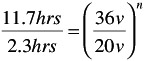
Therefore,

n = 2.767

Now we can use the following equation to determine the characteristic life at 5 volts:

_u = _a [Accelerated stress/Rated stress] ⁿ
₅ _v = ₃₆ _v [Accelerated stress/Rated stress] ⁿ = 2.3 = 542 hours

The characteristic life at 5 volts is 542 hours.

The reader must be very careful here because not all electronic parts or assemblies will follow the inverse power law model. Therefore, its applicability must usually be verified experimentally before use.

Arrhenius Model

The Arrhenius relationship for reaction rate is often used to account for the effect of temperature on electrical/electronic components. The Arrhenius relationship is as follows :

Reaction rate = A exp

where: A = normalizing constant; K _B = Boltzman's constant (8.63 — 10 ^-5 ev/degrees K); T = ambient temperature in degrees Kelvin; and E _a = activation energy type constant (unique for each failure mechanism).

In those situations where it can be shown that the failure mechanism rate follows the Arrhenius rate with temperature, the following Acceleration Factor (AF) can be developed:

Rate _use = A exp

Rate _accelerated = A exp

Acceleration Factor = AF = Rate _a /Rate _u =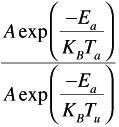

where T _a = acceleration test temperature in degrees Kelvin and T _u = actual use temperature in degrees Kelvin.

Assume we have a device that has an activation energy of 0.5 and a characteristic life of 2750 hours at an accelerated operating temperature of 150 °C. We want to find the characteristic life at an expected use temperature of 85 °C. (Remember that the conversion factor for Celsius to Kelvin is: °K = °C + 273 ” You may want to review Volume II.)

Therefore:

T _a = 150 + 273 = 423 °K and T _u = 85 + 273 = 358 °K

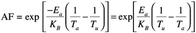
The E _a = 0.5. Our calculations would look like:

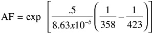
AF = exp [2.49] = 12. Therefore, the acceleration factor is 12. To determine life at 85 °C, multiply the acceleration factor times the characteristic life at the accelerated test level of 150 °C.

Characteristic life at 85 °C = (12) (2750 hours) = 33,000 hours