TYPICAL RM MEASURES

TYPICAL R&M MEASURES

R&M MATRIX

Perhaps the most important document in the R&M process is the R&M matrix. This matrix identifies the requirements of the customer on a per phase basis. Three major categories of tasks are usually identified. They are:

R&M programmatic tasks
Engineering tasks
R&M continuous improvement

RELIABILITY POINT MEASUREMENT

This may be expressed by:

R ₍ _t ₎ =

where R(t) = reliability point estimate during a constant failure rate period; e = natural logarithm which is 2.718281828...; t = schedule time or mission time of the equipment or machinery; and MTBF = mean time between failure.

Special note:

This calculation may be performed only when the machine has reached the bottom of the bathtub curve.

A water pump is scheduled (mission time) to operate for 100 hours. The MTBF for this pump is also rated at 100 hours and the MTTR is 2 hours. The probability that the pump will not fail during the mission is:

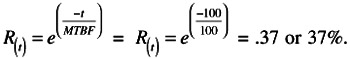
This means that the pump will have a 37% chance of not breaking down during the 100- hour mission time.

Conversely, the unreliability of the pump can be calculated as:

= 1 - R = 1 - .37 = .63 or 63%.

This means that the pump has a 63% chance of failing during the 100 hour mission.

MTBE

Mean time between event can be calculated as:

MTBE = Total Operating Time/N

where Total Operating Time = the total scheduled production time when machinery or equipment is powered and producing parts and N = the total number of downtime events, scheduled and unscheduled.

The total operating time for a machine is 550 hours. In addition, the machine experiences 2 failures, 2 tool changes, 2 quality checks, 1 preventive maintenance meeting, and 5 lunch breaks. What is the MTBE?

MTBE = Total Operating Time/N = 550/12 = 45.8 hours

MTBF

Mean time between failure is the average time between failure occurrences and is calculated as:

MTBF = Operating Time/N

where Operating Time = scheduled production time and N = total number of failures observed during the operating period.

If machinery is operating for 400 hours and there are eight failures, what is the MTBF?

MTBF = Operating Time/N = 400/8 = 50 hours. (Special note: Sometimes C (cycles) is substituted for T. In that case, we calculate the MCBF. The steps are identical to those of the MTBF calculation.)

FAILURE RATE

Failure rate estimates the number of failures in a given unit of time, events, cycles, or number of parts. It is the probability of failure within a unit of time. It is calculated as:

Failure rate = 1/MTBF

The failure rate of a pump that experiences one failure within an operating time period of 2000 hours is:

Failure rate = 1/MTBF = 1/2000 = .0005 failures per hour.

This means that there is a .0005 probability that a failure will occur with every hour of operation.

MTTR

Mean time to repair is a calculation based on one failure and one failure only. The longer each failure takes to repair, the more the equipment's cost of ownership goes up. Additionally, MTTR directly effects uptime, uptime percent, and capacity. It is calculated as:

MTTR =

where = total repair time and N = total number of repairs .

A pump operates for 300 hours. During that period there were four failure events recorded. The total repair time was 5 hours. What is the MTTR?

MTTR = = 5/4 = 1.25 hours

AVAILABILITY

Availability is the measure of the degree to which machinery or equipment is in an operable and committable state at any point in time. Availability is dependent upon (a) breakdown loss, (b) setup and adjustment loss, and (c) other factors that may prevent machinery from being available for operation when needed. When calculating this metric, it is assumed that maintenance starts as soon as the failure is reported . (Special note: Think of the measurement of R&M in terms of availability. That is, MTBF is reliability and MTTR is maintainability.) Availability is calculated as:

Availability = MTBF/(MTBF + MTTR)

What is the availability for a system that has an MTBF of 50 hours and an MTTR of 1 hour?

Availability = MTBF/(MTBF + MTTR) = 50/(50 + 1) = .98 or 98%

OVERALL EQUIPMENT EFFECTIVENESS (OEE)

Overall equipment effectiveness (OEE) is a measure of three variables . They are:

Availability = percent of time a machine is available to produce
Performance efficiency = actual speed of the machine as related to the design speed of the machine
Quality rate = percent of resulting parts that are within specifications

A good OEE is considered to be 85% or higher.

LIFE CYCLE COSTING (LCC)

Life cycle costing (LCC) is the total cost over the life of the machine or equipment. It is calculated based on the following:

LCC = Acquisition costs (A) + Operating costs (O) + Maintenance costs (M) ± Conversion and or decommission costs (c)

What is the LCC for the two machines shown in Table 8.2 and which one is a better deal?

Table 8.2: Cost Comparison of Two Machines
Costs	Machine A	Machine B
Acquisition costs (A)	$2,000.00	$1,520.00
Operating costs (O)	$9,360.00	$10,870.00
Maintenance costs (M)	$7,656.00	$9,942.00
Conversion and/or decommission costs (C)
Total LCC	$19,016.00	$22,332.00

The reader should notice that before the decision is made all costs should be evaluated. In this case, machine A has a higher acquisition cost than machine B, but it turns out that machine A has a lower LCC than machine B. Therefore, machine A is the better deal.

THERMAL ANALYSIS

This analysis is conducted to help the designer to develop the appropriate and applicable heat transfer (Table 8.3). The actual analysis is conducted by following these six steps:

Develop a list of all electrical components in the enclosure.
Identify the wattage rating for each component located in the enclosure.
Sum the total wattage for the enclosure.
Add in any external heat generating sources.
Calculate the surface area of the enclosure that will be available for cooling.
Calculate the thermal rise above ambient.

Table 8.3: Thermal Calculation Values
Thermal Calculation Values
Component Name	Quantity	Individual Wattage Maximum	Total Wattage
Internal
Relay	4	2.5	10.0
A18 contactor	1	1.7	1.7
A25 contactor	2	2	4.0
PS27 power supply	1	71	71.0
Monochrome monitor	1	85	85.0
		Subtotal wattage	171.7
External
Servo transformer	1	450	63.0
		Subtotal wattage	63.0
		Total enclosure wattage	234.7
Note: The servo transformer is mounted externally and next to the enclosure. Therefore, only 14% of the total wattage is estimated to radiate into the enclosure

The electrical enclosure is 5 ft. tall by 4 ft. deep. The surface area for this enclosure is calculated as follows :

Front and Back	=	5 ft. — 4ft. — 2 = 40 sq. ft.
Sides	=	2 ft. — 5 ft. — 2 = 20 sq. ft.
Enclosure top	=	2ft. — 4ft. = 8 sq. ft

Bottom is ignored due to the fact that heat rises.

Total surface area = 40 + 20 + 8 = 68 sq. ft.

To calculate the thermal rise (AT) we use the following formula:

Thermal rise (AT) = Thermal resistance ( _CA ) cabinet to ambient — Power (W)

_CA = 1/(Thermal conductivity — Cooling area)

The thermal conductivity value is found in the catalog of the National Electrical Manufacturing Association (NEMA).

_CA	=	1/(.25 W/degree F) — (square footage)
_CA	=	1/.25 — 68 = .0588

Thus, .25 W/degree F is the thermal conductivity value for a NEMA 12 enclosure. If the equipment inside the enclosure generates 234.7 watts, then the thermal rise is

ˆ T = _CA — wattage = .0588 — 234.7 = 13.8 °F.

If the ambient temperature is 100 °F, then the enclosure temperature will reach 113.8 °F. If the enclosure temperature is specified as 104 °F, then the design exceeds the specification by approximately 9.8 °F. The enclosure must be increased in size , the load must be reduced, or active cooling techniques need to be applied. ( Special note: Remember that a 10% rise in temperature decreases the reliability by about 50%. Also the method just mentioned in this example is not valid for enclosures that have other means of heat dissipation such as fans, or for those made of heavier metal or if the material were changed. This specific calculation assumes that the heat is being radiated through convection to the outside air.)

ELECTRICAL DESIGN MARGINS

Design margins in electrical engineering of the equipment are referred to as derating. On the other hand, mechanical design margins are referred to as safety margins. A rule of thumb for derating is about 20% for electrical components. However, the actual calculation is

% derating = 1 -

where I _T = total circuit current draw and I _s = total supply current.

During a design review, the question arose as to whether the 24 V power supply for a motor was adequately derated. The power supply takes 480 VAC three phase with a 2 A circuit breaker and has a rated output of 10 A. An examination of the system reveals that 24 V power is delivered to the load through three circuit breakers (A = .477 A, B = .73 A, and C = 5.53 A. The total for the three circuits is therefore 6.737 A.) When these circuit breakers are combined, 11 A of current flow to the load. This situation may not happen, but further investigation is required.

This means that in this case the power supply will not be overloaded and the circuit breakers are generously oversized. In other words, the circuit breakers should not be tripped due to false triggers.

SAFETY MARGINS (SM)

For mechanical components, SM are generally defined as the amount of strength of a mechanical component relating to the applied stress. A rule of thumb for SM with a normally distributed stress load relationship is that the safety margin should always be greater or equal to three. However, the actual calculation for the MS is

SM =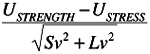

Where SM = safety margin; U _STRENGTH = mean strength; U _LOAD = mean load; Lv ² = load variance; and Sv ² = strength variance.

A robot's arm has a mean strength of 80 kg. The maximum allowable stress applied by the end of arm tooling is 50 kg. The strength variance is 8 kg and the stress variance is 7 kg. What is the SM?

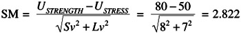
(A low SM may indicate the need to assign another size robot or redesign the tooling material.)

INTERFERENCE

Once the SM is calculated, it can be used to calculate the interference and reliability of the components under investigation. Interference may be thought of as the overlap between the stress and the strength distributions. In more formal terms, it is the probability that a random observation from the load distribution exceeds a random observation from the strength distribution. To calculate interference, we use the SM equation and substitute the z for the SM distribution:

Z =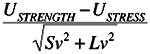

If we use the answer from the previous example (z = 2.822), we can use the z table (in this case the area under the z = 2.822 is .0024). This means that there exists a .0024 or .24% probability of failure.

Reliability, on the other hand, may be calculated as

R	=	1 - interference or R = 1 - ±
R	=	1 - .0024 = .9976 or 99.76%.

This means that even though the strength and the load have a very low (.24%) probability of failure, the reliability of the system is very high with a 99.76%.

CONVERSION OF MTBF TO FAILURE RATE AND VICE VERSA

The relationship between these two metrics is

RELIABILITY GROWTH PLOTS

This plot is an effective method to track continual improvement for R&M as well as to predict reliability growth of machinery from one machine to the other. The steps to generate this plot are:

Step 1. Collect data on the machine and calculate the cumulative MTBF value for the machine.
Step 2. Plot the data on log-log paper. (An increasing slope indicates a reliability growth flatness , which indicates that the machine has achieved its inherent level of MTBF and cannot get any better)

Step 3. Calculate the slope, using regression analysis or best fit line. Once the slope (the beta value) is calculated, we can apply the Duane model interpretation. The guidelines (Table 8.4) for the interpretation are

Table 8.4: Guidelines for the Duane Model
²	Recommended Actions
0 to .2	No priority is given to reliability improvement; failure data not analyzed ; corrective action taken for important failure modes, but with low priority
.2 to .3	Routine attention to reliability improvement; corrective action taken for important failure modes
.3 to .4	Priority attention to reliability improvement; normal (typical stresses) environment utilization; well-managed analysis and corrective action for important failure modes
.4 to .6	Eliminating failures takes top priority; immediate analysis and corrective action for all failures

MACHINERY FMEA

Machinery FMEA is a systematic approach that applies the tabular method to aid the thought process used by simultaneous engineering teams to identify the machine's potential failure modes, potential effects, and potential causes and to develop corrective action plans that will remove or reduce the impact of the failure modes. Perhaps the most important use of the machinery FMEA is to identify and correct all safety issues. A more detailed discussion will be given in Chapter 6.