Transact-SQL Programming Constructs--The Basics
Transact-SQL extends standard SQL by adding many useful programming constructs. These constructs will look familiar to developers experienced with C/C++, Basic/Microsoft Visual Basic, Fortran, Java, Pascal, and similar languages. The Transact-SQL extensions are wonderful additions to the original SQL standard. Before the extensions were available, requests to the database were always simple, single statements. Any conditional logic had to be provided by the calling application. With a slow network or via the Internet, this would be disastrous, requiring many trips across the network ”more than are needed by simply letting conditions be evaluated at the server and allowing subsequent branching of execution.
Variables
Without variables, a programming language wouldn't be particularly useful; Transact-SQL is no exception. Variables that you declare are local variables, having scope and visibility only within the batch or stored procedure in which you declare them. (The next chapter discusses the details of batches and stored procedures.) In code, the single @ character designates a local variable.
Transact-SQL has no true global variables. Older documentation refers to certain parameterless system functions as global variables because they're designated by @@ , which is similar to the designation for local variables. We'll look at these in a little more detail at the end of the chapter, in the section on system functions.
User -declared global variables would be a nice enhancement that we might see in a future release. Until then, temporary tables provide a decent alternative for sharing values among connections.
Local Variables
You declare local variables at the beginning of a batch or a stored procedure. (The batch or stored procedure can be part of a transaction as well.) You can subsequently assign values to local variables either with the SELECT statement or the SET statement, using an equal (=) operator. The values you assign using the SET statement can be constants, other variables, or expressions. When assigning to a variable using a SELECT statement, the values to be assigned are typically selected from a column in a table. The syntax for declaring and using the variables is identical, regardless of the method you use to assign the values to the variable. In the following example, we declare a variable, assign it a value using the SET statement, and then use that variable in a WHERE clause:
DECLARE @limit money SET @limit = SELECT * FROM titles WHERE price <= @limit |
We could have written the same code using the SELECT statement instead of the SET statement. However, you typically use SELECT when the values to be assigned are found in a column of a table. A SELECT statement used to assign values to one or more variables is called an assignment SELECT . You can't combine the functionality of the assignment SELECT and a "regular" SELECT in the same statement. That is, if a SELECT statement is used to assign values to variables, it can't also return values to the client as a result set. In the following simple example, we declare two variables, assign values to them from the roysched table, and then select their values as a result set.
DECLARE @min_range int, @hi_range int -- Variables declared SELECT @min_range=MIN(lorange), @hi_range=MAX(hirange) FROM roysched -- Variables assigned SELECT @min_range, @hi_range -- Variables returned |
Note that a single DECLARE statement can declare multiple variables. When using a SELECT statement for assigning values, we can assign more than one value at a time. When using SET to assign values to variables, we must use a separate SET statement for each variable. For example, the following SET statement will return an error:
SET @min_range = 0, @hi_range = 100 |
Be careful when assigning variables by selecting a value from the database ”you want to ensure that the SELECT statement will return only one row. It's perfectly legal to assign a variable to a SELECT statement that will return multiple rows, but the variable's value probably isn't what you expect: no error message is returned, and the variable has the value of the last row returned.
For example, suppose that the following stor_name values exist in the stores table of the pubs database:
stor_name --------- Eric the Read Books Barnum's News & Brews Doc-U-Mat: Quality Laundry and Books Fricative Bookshop Bookbeat |
The following assignment runs without error but is probably a mistake:
DECLARE @stor_name varchar(30) SELECT @stor_name=stor_name FROM stores |
The resulting value of @stor_name is the last row, Bookbeat . But consider the order returned, without an ORDER BY clause, as a chance occurrence. Assigning a variable to a SELECT statement that returns more than one row usually wouldn't be intended, and it's probably a bug introduced by the developer. To avoid this situation, you should qualify the SELECT statement with an appropriate WHERE clause to limit the result set to the one row that meets your criteria.
Alternatively, you can use an aggregate function, such as MAX(), MIN(), or SUM(), to limit the number of rows returned. Then you can select only the value you want. If you want the assignment to be to only one row of a SELECT statement that might return many rows (and it's not important which row that is), you should at least use SET ROWCOUNT 1 or SELECT TOP 1 to avoid the effort of gathering many rows, with all but one row thrown out. (In this case, the first row would be returned, not the last. You could use ORDER BY to explicitly indicate which row should be first.) You might also consider checking the value of @@ROWCOUNT immediately after the assignment and, if it's greater than 1, branch off to an error routine.
Also be aware that if the SELECT statement assigning a value to a variable doesn't return any rows, nothing will be assigned. The variable will keep whatever value it had before the assignment SELECT statement was run. For example, suppose we use the same variable twice to find the first names of authors with a particular last name :
DECLARE @firstname varchar(20) SELECT @firstname = au_fname FROM authors WHERE au_lname = 'Greene' SELECT @firstname -- return the first name as a result SELECT @firstname = au_fname FROM authors WHERE au_lname = 'Delaney' SELECT @firstname -- return the first name as a result |
If you run the previous code, you'll see the same first name returned both times, because no authors with the last name of Delaney exist, at least not in the pubs database!
You can also assign a value to a variable in an UPDATE statement. This approach can be useful and more efficient than using separate statements to swap values. For example, suppose that in the jobs table, we realize the min and max columns have accidentally been reversed . The following UPDATE statement efficiently swaps all the values. (To run this example, you must disable the CHECK constraints on the min_lvl and max_lvl columns.)
DECLARE @tmp_val tinyint BEGIN TRAN UPDATE jobs SET @tmp_val=min_lvl, min_lvl=max_lvl, max_lvl=@tmp_val |
Control-of-Flow Tools
Like any programming language worth its salt, Transact-SQL provides a decent set of control-of-flow tools. (True, Transact-SQL has only a handful of tools, perhaps not as many as you'd like, but they're enough to make it dramatically more powerful than standard SQL.) The control-of-flow tools include condi- tional logic (IF...ELSE and CASE), loops (only WHILE, but it comes with CONTINUE and BREAK options), unconditional branching (GOTO), and the ability to return a status value to a calling routine (RETURN). Table 9-1 presents a quick summary of these control-of-flow constructs, which you'll see used at various times in this book.
Table 9-1. Control-of-flow constructs in Transact-SQL.| Construct | Description |
|---|---|
| BEGIN...END | Defines a statement block. Using BEGIN...END allows a group of statements to be executed. Typically, BEGIN immediately follows IF, ELSE, or WHILE. ( Otherwise , only the next statement will be executed.) For C programmers, BEGIN...END is similar to using a {..} block after IF. |
| GOTO label | Continues processing at the statement following the specified label. |
| IF...ELSE | Defines conditional and, optionally , alternate execution when a condition is false. |
| RETURN [ n ] | Exits unconditionally. Typically used in a stored procedure or trigger (although it can also be used in a batch). Optionally, a whole number n (positive or negative) can be set as the return status, which can be assigned to a variable when executing the stored procedure. |
| WAITFOR | Sets a time for statement execution. The time can be a delay interval (up to 24 hours) or a specific time of day. The time can be supplied as a literal or with a variable. |
| WHILE | The basic looping construct for SQL Server. Repeats a statement (or block) while a specific condition is true. |
| ...BREAK | Exits the innermost WHILE loop. |
| ...CONTINUE | Restarts a WHILE loop. |
CASE
The CASE expression is enormously powerful. Although CASE is part of the ANSI SQL-92 specification, it's not required for ANSI compliance certification, and few products other than Microsoft SQL Server have implemented it. If you have experience with an SQL database system other than Microsoft SQL Server, chances are you haven't used CASE. If that's the case (pun intended), you should get familiar with it now. It's time well spent. CASE was added in version 6.0, and once you get used to using it, you'll wonder how SQL programmers ever managed without it.
CASE is a conceptually simpler way to do IF-ELSE IF-ELSE IF-ELSE IF-ELSE_type operations. It's roughly equivalent to a switch statement in C. However, CASE is far more than a shorthand for IF ”in fact, it's not really even that. CASE is an expression, not a control-of-flow keyword, which means that it can be used only inside other statements. You can use CASE in a SELECT statement in the SELECT list, in a GROUP BY clause, or in an ORDER BY clause. You can use it in the SET clause of an UPDATE statement. You can include CASE in the values list for an INSERT statement. You can also use CASE in a WHERE clause in any SELECT, UPDATE, or DELETE statement. Anywhere that T-SQL expects an expression, you can use CASE to determine the value of that expression.
Here's a simple example of CASE. Suppose that we want to classify books in the pubs database by price. We want to segregate them as low priced, moderately priced, or expensive. And we'd like to do this with a single SELECT statement and not use UNION. Without CASE, we can't do it. With CASE, it's a snap:
SELECT title, price, 'classification'=CASE WHEN price < 10.00 THEN 'Low Priced' WHEN price BETWEEN 10.00 AND 20.00 THEN 'Moderately Priced' WHEN price > 20.00 THEN 'Expensive' ELSE 'Unknown' END FROM titles |
Notice that even in this example, we need to worry about NULL, because a NULL price won't fit into any of the category buckets.
Following are the abbreviated results.
title price classification ------------------------------------- ------ ----------------- The Busy Executive's Database Guide 19.99 Moderately Priced Cooking with Computers: Surreptitious 11.95 Moderately Priced Balance Sheets You Can Combat Computer Stress! 2.99 Low Priced Straight Talk About Computers 19.99 Moderately Priced Silicon Valley Gastronomic Treats 19.99 Moderately Priced The Gourmet Microwave 2.99 Low Priced The Psychology of Computer Cooking NULL Unknown But Is It User Friendly? 22.95 Expensive |
If all the conditions after your WHEN clauses are equality comparisons against the same value, you can use an even simpler form so that you don't have to keep repeating the expression. Suppose we want to print the type of each book in the titles table in a slightly more user-friendly fashion ”for example, Modern Cooking instead of mod_cook . We could use the following SELECT statement:
SELECT title, price, 'Type' = WHEN type = 'mod_cook' THEN 'Modern Cooking', WHEN type = 'trad_cook' THEN 'Traditional Cooking' WHEN type = 'psychology' THEN 'Psychology' WHEN type = 'business' THEN 'Business' WHEN type = 'popular_comp' THEN 'Popular Computing' ELSE 'Not yet decided' END FROM titles |
In this example, because every condition after WHEN is testing for equality with the value in the type column, we can use an even simpler form. You can think of this simplification as factoring out the type = from every WHEN clause, and place the type column at the top of the CASE expression:
SELECT title, price, 'Type' = type WHEN 'mod_cook' THEN 'Modern Cooking', WHEN 'trad_cook' THEN 'Traditional Cooking' WHEN 'psychology' THEN 'Psychology' WHEN 'business' THEN 'Business' WHEN 'popular_comp' THEN 'Popular Computing'' ELSE 'Not yet decided' END FROM titles |
You can use CASE in some unusual places; because it's an expression, you can use it anywhere an expression is legal. Using CASE in a view is a nice technique that can make your database more usable to others. For example, in Chapter 7, we saw CASE in a view using CUBE to shield users from the complexity of "grouping NULL" values. Using CASE in an UPDATE statement can make the update easier. More importantly, CASE can allow you to make changes in a single pass of the data that would otherwise require you to do multiple UPDATE statements, each of which would have to scan the data.
The Transact-SQL documentation for the previous version of SQL Server (6.5) had a nice conceptual example that we've reproduced here. Although it works fine and illustrates CASE, we've rewritten the UPDATE statement with an equivalent formulation that might be more intuitive.
-- In this example, reviews have been turned in and big salary -- adjustments are due. A review rating of 4 will double the -- worker's salary, 3 will increase it by 60 percent, 2 will -- increase it by 20 percent, and a rating lower than 2 will -- result in no raise. A raise will not be given if the employee -- has been at the company for less than 18 months. UPDATE employee_salaries SET salary= CASE WHEN (review=4 AND (DATEDIFF(month, hire_date, GETDATE()) >= 18)) THEN salary * 2.0 WHEN (review=3 AND (DATEDIFF(month, hire_date, GETDATE()) >= 18)) THEN salary * 1.6 WHEN (review=2 AND (DATEDIFF(month, hire_date, GETDATE()) >= 18)) THEN salary * 1.2 ELSE salary END -- This second formulation produces identical results, but it's _ more intuitive and clearer UPDATE employee_salaries SET salary= CASE review WHEN 4 THEN salary * 2.0 WHEN 3 THEN salary * 1.6 WHEN 2 THEN salary * 1.2 ELSE salary END WHERE (DATEDIFF(month, hire_date, GETDATE()) > 18) |
Cousins of CASE
SQL Server provides three nice shorthand derivatives of CASE: COALESCE, NULLIF, and ISNULL. COALESCE and NULLIF are both part of the ANSI SQL-92 specification; they were added to version 6.0 at the same time that CASE was added. ISNULL() is a longtime SQL Server function. Following is the syntax for these functions.
COALESCE This function is equivalent to a CASE expression that returns the first NOT NULL expression in a list of expressions.
COALESCE( expression1 , expression2 , ... expressionN ) |
If no non-null values are found, COALESCE returns NULL (which is what expressionN was, given that there were no non-null values). Written as a
CASE expression, COALESCE looks like this:
CASE WHEN expression1 IS NOT NULL THEN expression1 WHEN expression2 IS NOT NULL THEN expression2 ELSE expressionN END |
NULLIF This function is equivalent to a CASE expression in which NULL is returned if expression1 = expression2 .
NULLIF( expression1 , expression2 ) |
If the expressions aren't equal, expression1 is returned. In Chapter 7, you saw that NULLIF can be handy if you use dummy values instead of NULL, but you don't want those dummy values to skew the results produced by aggregate functions. Written using CASE, NULLIF looks like this:
CASE WHEN expression1 = expression2 THEN NULL ELSE expression1 END |
ISNULL This function is almost the mirror of NULLIF.
ISNULL( expression1 , expression2 ) |
ISNULL allows you to easily substitute an alternative expression or value for an expression that's NULL. In Chapter 7, we saw the use of ISNULL to substitute the string ' ALL ' for a grouping NULL when using CUBE and to substitute a string of question marks, ' ???? ' for a NULL value. By doing this, the results were more clear and intuitive to users. Written instead using CASE, ISNULL looks like this:
CASE WHEN expression1 IS NULL THEN expression2 ELSE expression1 END |
The second argument to ISNULL (the value to be returned if the first argument is NULL) can be an expression or even a SELECT statement. Say, for example, that we want to query the titles table. If a title has NULL for price, we want to instead use the lowest price that exists for any book. Without CASE or ISNULL, this isn't an easily written query. With ISNULL, it is easy:
SELECT title, pub_id, ISNULL(price, (SELECT MIN(price) FROM titles)) FROM titles |
For comparison, here's an equivalent SELECT statement written with the longhand CASE formulation:
SELECT title, pub_id, CASE WHEN price IS NULL THEN (SELECT MIN(price) FROM titles) ELSE price END FROM titles |
Transact-SQL, like other programming languages, provides printing capability through the PRINT and RAISERROR statements. We'll discuss RAISERROR momentarily, but first we'll take a look at the PRINT statement.
PRINT is the most basic way to display any character string up to 8000 characters . You can display a literal character string or a variable of type char , varchar , nchar , nvarchar , datetime , or smalldatetime . You can concatenate strings and use functions that return string or date values. In addition, PRINT can print any expression or function that is implicitly convertible to a character datatype. (Refer to Table 9-10 to determine which datatypes are implicitly convertible .)
It seems like every time you learn a new programming language, the first assignment is to write the "Hello World" program. Using TRANSACT-SQL, it couldn't be easier:
PRINT 'Hello World' |
Even before we saw PRINT, you could've produced the same output in your Query Analyzer screen with the following:
SELECT 'Hello World' |
So what's the difference between the two? The PRINT returns a message, nothing more. The SELECT statement returns output like this:
----------- Hello World (1 row(s) affected) |
The SELECT statement returns the string as a result set. That's why we get the (1 row(s) affected) message. When using the Query Analyzer to submit your queries and view your results, you might not see much difference between the PRINT and the SELECT statements. But for other client tools (besides ISQL, OSQL, and Query Analyzer), there could be a big difference. PRINT returns a message of severity 0, and you need to check the documentation for the client API that you're using to determine how messages are handled. For example, if you're writing an ODBC program, the results of a PRINT statement get handled by SQLError() .
On the other hand, a SELECT statement returns a set of data, just like selecting prices from a table. Your client interface might expect you to bind data to local (client-side) variables before you can use them in your client programs. Again, you'll have to check your documentation to know for sure. The important distinction to remember here is that PRINT returns a message and SELECT returns data.
PRINT is extremely simple, both in its use and in its capabilities. It's not nearly as powerful as, say, printf() in C. You can't give positional parameters or control formatting. For example, you can't do this:
PRINT 'Today is %s', GETDATE() |
Part of the problem here is that %s is meaningless. In addition, the built-in function GETDATE() returns a value of type datetime , which can't be concatenated to the string constant. So, we can do this instead:
PRINT 'Today is ' + convert(char(30), GETDATE()) |
RAISERROR
RAISERROR is similar to PRINT but can be much more powerful than it. RAISERROR also sends a message (not a result set) to the client; however, i t allows you to specify the specific error number and severity of the message. It also allows you to reference an error number, the text for which you can add to the sysmessages table. RAISERROR makes it easy for you to develop international versions of your software. Rather than have multiple versions of your SQL code when you want to change the language of the text, you need only one version. You can simply add the text of the message in multiple languages. The user will see the message in the language used by the particular connection.
Unlike PRINT, RAISERROR accepts printf -like parameter substitution as well as formatting control. RAISERROR also can allow messages to be logged to the Windows NT event service, making them visible to the Windows NT event viewer, and it allows SQL Server Agent alerts to be configured for these events. In many cases, RAISERROR is preferable to PRINT, and you might choose to use PRINT only for quick-and-dirty situations. For production-caliber code, RAISERROR is usually a better choice. Here's the syntax:
RAISERROR ({ msg_id msg_str }, severity , state [, argument1 [, argument2 ]]) [WITH LOG] |
After calling RAISERROR, the system function @@ERROR will return the value passed as msg_id . If no ID is passed, the error is raised with error number 50000, and @@ERROR will be set to that number. You can also set the severity level; an informational message should be considered severity 0 (or severity 10; 0 and 10 are used interchangeably for a historical reason that's not important). Only someone with the system administrator (SA) role can raise an error with a severity of 19 or higher. Errors of severity 20 and higher are considered fatal, and the connection to the client will automatically be terminated .
You must use the WITH LOG option for all errors of severity 19 or higher. For errors of severity 20 or higher, the message text isn't returned to the client. Instead, it's sent to the SQL Server error log, and the error number, text, severity, and state are written to the Windows NT event log. The SA can use the WITH LOG option with any error number or any severity level.
Errors written to the Windows NT event log from RAISERROR go to the application event log, with MSSQLServer as the source and Server as the category. These errors have event ID 17060. (Errors that SQL Server raises can have different event IDs, depending on which component they come from.) The type of message in the Windows NT event log depends on the severity used in the RAISERROR statement. Messages with severity 14 and lower are recorded as informational messages, severity 15 messages are warnings, and severity 16 and higher messages are errors . Note that the severity that's recorded in the event log is the number that's passed to RAISERROR, regardless of the stated severity in sysmessages . So, although we don't recommend it, you can raise a serious message as informational or a noncritical message as an error. If you look at the data section of the Windows NT event log for a message raised from RAISERROR, or if you're reading from it in a program, you'll notice that the error number appears first, followed by the severity level.
You can use any number from 1 through 127 as the state parameter. You might pass a line number that tells where the error was raised. But state has no real relevance to SQL Server.
TIP
There's a little-known way to cause isql.exe or OSQL.EXE (the command-line query tools) to terminate. Raising any error with state 127 causes isql or OSQL to immediately exit, with a return code equal to the error number. (You can determine the error number from a batch command file with ERRORLEVEL.) You could write your application so that it does something similar ”it's a simple change to the error-handling logic. This trick can be a useful way to terminate a set of scripts that would be run through isql or OSQL. You could get a similar result by raising a high-severity error to terminate the connection. But using a state of 127 is actually simpler, and no scary message will be written to the error log or event log for what is a planned, routine action.
You can add your own messages and text for a message in multiple languages by using the sp_addmessage stored procedure. By default, SQL Server uses U.S. English, but you can add languages. (SQL Server distinguishes U.S. English from British English because of locale settings, such as currency. The text of messages is the same.) The script \mssql7\install\instlang.sql adds locale settings for nine more languages but not the actual translated messages. Error numbers lower than 50000 are reserved for SQL Server use, so choose a higher number for your own messages.
Suppose we want to rewrite "Hello World" to use RAISERROR, and we want the text of the message to be able to appear in both U.S. English and German (language ID of 1). Here's how:
EXEC sp_addmessage 50001, 10, 'Hello World', @replace='REPLACE' -- New message 50001 for U.S. English EXEC sp_addmessage 50001, 10, 'Hallo Welt' , @lang='Deutsch', @replace='REPLACE' -- New message 50001 for German |
When RAISERROR is executed, the text of the message becomes dependent on the SET LANGUAGE setting of the connection. If the connection does a SET LANGUAGE Deutsch , the text returned for RAISERROR (50001, 10, 1) will be Hallo Welt . If the text for a language doesn't exist, the U.S. English text (by default) will be returned. For this reason, the U.S. English message must be added before the text for another language is added. If no entry exists, even in U.S. English, error 2758 results:
Msg 2758, Level 16, State 1 RAISERROR could not locate entry for error n in Sysmessages. |
We could easily enhance the message to say whom the "Hello" is from by providing a parameter marker and passing it when calling RAISERROR. (For illustration, we'll use some printf -style formatting, #6x , to display the process number in hexadecimal format.)
EXEC sp_addmessage 50001, 10, 'Hello World, from: %s, process id: %#6x', @replace='REPLACE' |
When user kalend executes
DECLARE @parm1 varchar(30), @parm2 int SELECT @parm1=USER_NAME(), @parm2=@@spid RAISERROR (50001, 15, -1, @parm1, @parm2) |
this error is raised:
Msg 50001, Level 15, State 1 Hello, World, from: kalend, process id: 0xc |
FORMATMESSAGE
If you have created your own error messages with parameter markers, you might need to inspect the entire message with the parameters replaced by actual values. RAISERROR makes the message string available to the client but not to your SQL Server application. To construct a full message string from a parameterized message in the sysmessages table, you can use the function FORMATMESSAGE().
If we consider the last example from the preceding RAISERROR section, we can use FORMATMESSAGE to build the entire message string and save it in a local variable for further processing. Here's an example of the use of FORMATMESSAGE:
DECLARE @parml varchar(30), @parm2 int, @message varchar(100) SELECT @parm1=USER_NAME(), @parm2=@@spid SELECT @message = FORMATMESSAGE(50001, @parm1, @parm2) PRINT 'The message is: ' + @message |
This will return the following:
The message is: Hello World, from: kalend, process id: Oxc |
Note that no error number or state information is returned.
Operators
Transact-SQL provides a large collection of operators for doing arithmetic, comparing values, doing bit operations, and concatenating strings. These operators are similar to those you might be familiar with in other programming languages. You can use Transact-SQL operators in any expression, including in the select list of a query, in the WHERE or HAVING clauses of queries, in UPDATE and IF statements, and in CASE expressions.
Arithmetic Operators
We won't go into much detail here because arithmetic operators are pretty standard stuff. If you need more information, please refer to the online documentation. Table 9-2 shows the arithmetic operators.
Table 9-2. Arithmetic operators in Transact-SQL.
| Symbol | Operation | Used with These Datatypes |
|---|---|---|
| + | Addition | int , smallint , tinyint , numeric , decimal , float , real , money , and smallmoney |
| - | Subtraction | int , smallint , tinyint , numeric , decimal , float , real , money , and smallmoney |
| * | Multiplication | int , smallint , tinyint , numeric , decimal , float , real , money , and smallmoney |
| / | Division | int , smallint , tinyint , numeric , decimal , float , real , money , and smallmoney |
| % | Modulo | int , smallint , and tinyint |
As with other programming languages, in Transact-SQL you need to consider the datatypes you're using when performing arithmetic operations, or you might not get the results you expect. For example, which of the following is correct?
1 · 2 = 0
1 · 2 = 0.5
If the underlying datatypes are both integers (including tinyint and smallint ), the correct answer is 0. If one or both of the datatypes are float (including real ) or numeric / decimal with a nonzero scale, the correct answer is 0.5 (or 0.50000, depending on the precision and scale of the datatype). When an operator combines two expressions of different datatypes, the datatype precedence rules specify which datatype is converted to the other. The datatype with the lower precedence is converted to the datatype with the higher precedence.
Here's the precedence order for SQL Server datatypes:
datetime (highest) smalldatetime float real decimal money smallmoney int smallint tinyint bit ntext text image timestamp nvarchar nchar varchar char varbinary binary uniqueidentifier (lowest) |
As you can see from the above precedence list, an int multiplied by a float produces a float . You can explicitly convert to a given datatype by using the CAST() function or its predecessor, CONVERT(). These conversion functions are discussed later in this chapter.
The addition (+) operator is also used to concatenate character strings. In this example, we want to concatenate last names, followed by a comma and a space, followed by first names from the authors table (in pubs ), and then return the result as a single column:
SELECT 'author'=au_lname + ', ' + au_fname FROM authors |
Here's the abbreviated result:
author ------ White, Johnson Green, Marjorie Carson, Cheryl O'Leary, Michael |
Bit Operators
Table 9-3 shows the SQL Server bit operators.
Table 9-3. SQL Server bit operators.
| Symbol | Meaning |
|---|---|
| & | Bitwise AND (two operands) |
| Bitwise OR (two operands) | |
| ^ | Bitwise exclusive OR (two operands) |
| ~ | Bitwise NOT (one operand) |
The operands for two-operand bitwise operators can be any of the datatypes of the integer or binary string datatype categories (except for the image datatype); however, neither operand can be any of the datatypes of the binary string datatype category. Table 9-4 shows the supported operand datatypes.
Table 9-4. Datatypes supported for two-operand bitwise operators.
| Left Operand | Right Operand |
|---|---|
| binary | int , smallint , or tinyint |
| bit | int , smallint , tinyint , or bit |
| int | int , smallint , tinyint , binary , or varbinary |
| smallint | int , smallint , tinyint , binary , or varbinary |
| tinyint | int , smallint , tinyint , binary , or varbinary |
| varbinary | int, smallint, or tinyint |
The single operand for the bitwise NOT operator must be one of the integer datatypes.
Often, you must keep a lot of indicator-type values in a database, and bit operators make it easy to set up bit masks with a single column to do this. The SQL Server system tables use bit masks. For example, the status field in the sysdatabases table is a bit mask. If we wanted to see all databases marked as read-only, which is the tenth bit or decimal 1024 (2 10 ), we could use this query:
SELECT "read only databases"=name FROM master..sysdatabases WHERE status & 1024 > 0 |
This example is for illustrative purposes only. In general, you shouldn't query the system catalogs directly. Sometimes the catalogs need to change between product releases, and if you query directly, your applications can break because of these required changes. Instead, you should use the provided system catalog stored procedures and object property functions, which return catalog information in a standard way. If the underlying catalogs change in subsequent releases, the property functions are also updated, insulating your application from unexpected changes.
So for this example, to see whether a particular database was marked read-only, we could use the DATABASEPROPERTY function:
SELECT DATABASEPROPERTY('mydb', 'IsReadOnly') |
A value of 1 returned would mean that mydb was set to read-only status.
Note that keeping such indicators as bit datatype columns can be a better approach than using an int as a bit mask. This approach is more straightforward ”you don't always need to look up your bit-mask values for each indicator. To write the query above, you'd need to check the documentation for the bit-mask value for "read only." And many developers, not to mention end users, aren't that comfortable using bit operators and are likely to use them incorrectly. From a storage perspective, bit columns don't require more space than creating equivalent bit-mask columns requires. (Eight bit fields can share the same byte of storage.)
True, bit columns have a couple of restrictions that you don't have if you create a bit mask as an integer and use bit operators: for example, you can't create an index on a bit column. But you wouldn't typically want to do that with a "yes/no" indicator field anyway. If you have a huge number of indicator fields, using bit-mask columns of integers instead of bit columns might be a better alternative than dealing with hundreds of individual bit columns. However, there's nothing to stop you from having hundreds of bit columns. You'd have to have an awful lot of bit fields to actually exceed the column limit, because a table in SQL Server can have up to 1024 columns. If you frequently add new indicators, using a bit mask on an integer might be better. To add a new indicator, you can make use of an unused bit of an integer status field rather than do an ALTER TABLE and add a new column (which you must do if you use a bit column). The case for using a bit column boils down to clarity.
Comparison Operators
Table 9-5 shows the SQL Server comparison operators.
Table 9-5. SQL Server comparison operators.
| Symbol | Meaning |
|---|---|
| = | Equal to |
| > | Greater than |
| < | Less than |
| >= | Greater than or equal to |
| <= | Less than or equal to |
| <> | Not equal to (ANSI standard) |
| != | Not equal to (not ANSI standard) |
| !> | Not greater than (not ANSI standard) |
| !< | Not less than (not ANSI standard) |
Comparison operators are straightforward. Only a couple of related issues might be confusing to a novice SQL Server developer:
- When dealing with NULL, remember the issues with three-value logic and the truth tables that were discussed in Chapter 7. Also understand that NULL is an unknown.
- Comparisons of char and varchar data (and their Unicode counterparts) depend on the sort order at the SQL Server installation. Whether comparisons evaluate to TRUE depends on the sort order installed. Review the discussion of sort orders in Chapter 4, "Planning for and Installing SQL Server"
Logical and Grouping Operators (Parentheses)
The three logical operators (AND, OR, and NOT) are vitally important in expressions, especially in the WHERE clause. You can use parentheses to group expressions and then apply logical operations to the group. In many cases, it's impossible to correctly formulate a query without using parentheses. In other cases, you might be able to avoid them, but it's not very intuitive and it could result in bugs . You could construct a convoluted expression using some combination of string concatenations or functions, bit operations, or arithmetic operations instead of using parentheses. But there's no good reason to do this.
Using parentheses can make your code clearer, less prone to bugs, and more easily maintained . Because there's no performance penalty beyond parsing, you should use parentheses liberally. Below is an example query that you couldn't readily write without using parentheses. This query is simple, and in English the request is well understood . But you're also likely to get this query wrong in Transact-SQL if you're not careful, and it clearly illustrates just how easy it is to make a mistake.
Find authors who do not live in either Salt Lake City, UT, or Oakland, CA. |
Following are four examples that attempt to formulate this query. Three of them are wrong. Test yourself: which one is correctly stated? (As usual, multiple correct formulations are possible ”not just the one presented here.)
EXAMPLE 1
SELECT au_lname, au_fname, city, state FROM authors WHERE city <> 'OAKLAND' AND state <> 'CA' OR city <> 'Salt Lake City' AND state <> 'UT' |
EXAMPLE 2
SELECT au_lname, au_fname, city, state FROM authors WHERE (city <> 'OAKLAND' AND state <> 'CA') OR (city <> 'Salt Lake City' AND state <> 'UT') |
EXAMPLE 3
SELECT au_lname, au_fname, city, state FROM authors WHERE (city <> 'OAKLAND' AND state <> 'CA') AND (city <> 'Salt Lake City' AND state <> 'UT') |
EXAMPLE 4
SELECT au_lname, au_fname, city, state FROM authors WHERE NOT ((city='OAKLAND' AND state='CA') OR (city='Salt Lake City' AND state='UT')) |
Hopefully, you can see that only Example 4 operates as wanted. This query would be impossible to write without some combination of parentheses, NOT, OR (including IN, a shorthand for OR), and AND. You can also use parentheses to change the order of precedence in mathematical and logical operations. These two statements return different results:
SELECT 1.0 + 3.0 / 4.0 -- Returns 1.75 SELECT (1.0 + 3.0) / 4.0 -- Returns 1.00 |
The order of precedence is similar to what you learned back in algebra class (except for the bit operators). Operators of the same level are evaluated left to right. You use parentheses to change precedence levels to suit your needs, when you're unsure, or when you simply want to make your code more readable. Groupings with parentheses are evaluated from the innermost grouping outward. Table 9-6 shows the order of precedence.
Table 9-6. Order of precedence, from highest to lowest.
| Operation | Operators |
|---|---|
| Bitwise NOT | ~ |
| Multiplication/division/modulo | * / % |
| Addition/subtraction | + ? |
| Bitwise exclusive OR | ^ |
| Bitwise AND | & |
| Bitwise OR | |
| Logical NOT | NOT |
| Logical AND | AND |
| Logical OR | OR |
If you didn't pick the correct example, you should easily see the flaw in Examples 1, 2, and 3 by examining the output. Both Examples 1 and 2 return every row. Every row is either not in CA or not in UT, because a row can be in only one or the other. A row in CA isn't in UT, so the expression returns TRUE. Example 3 is too restrictive ”for example, what about the rows in San Francisco, CA? The condition (city <> 'OAKLAND' and state <> 'CA') would evaluate as (TRUE and FALSE) for San Francisco, CA, which, of course, is FALSE, so the row would be rejected when it should be selected, according to the desired semantics.
Scalar Functions
In Chapter 7, we looked at aggregate functions, such as MAX(), SUM(), and COUNT(). These functions operate on a set of values to produce a single aggregated value. In addition to aggregate functions, SQL Server provides scalar functions, which operate on a single value. Scalar is just a fancy term for single value . You can also think of the value in a single column of a single row as scalar . Scalar functions are enormously useful ”the Swiss army knife of SQL Server. (You've probably noticed that scalar functions have been used in several examples already ”we'd all be lost without them.)
You can use scalar functions anywhere an expression is legal, such as:
- In the select list.
- In a WHERE clause, including one defining a view.
- Inside a CASE expression.
- In a CHECK constraint.
- In the VALUES clause of an INSERT statement.
- In an UPDATE statement to the right of the SET clause.
- With a variable assignment.
- As a parameter inside another scalar function.
SQL Server provides too many scalar functions to remember. The best you can do is to familiarize yourself with those that exist, and then, when you encounter a problem and a light bulb goes on in your head to remind you about a function that will help, you can look at the online documentation for details. Even with so many functions available, you'll probably find yourself wanting some functions that still don't exist. (And you probably still wouldn't be completely satisfied even if another couple hundred functions were added!) You might have a specialized need that would benefit from a specific function, and it would be great if we could write and add our own libraries of scalar functions.
Stored procedures and extended stored procedures come somewhat close and are extraordinarily useful, but even they fall short of the capability provided by scalar functions. And unlike scalar functions, stored procedures or extended stored procedures can't be used in a select list, in a view, or in a WHERE clause. But take heart ”the SQL Server developers do appreciate the need for user-defined functions, and no doubt user-defined functions will make their way into some future SQL Server release. Until then, familiarize yourself with the functions provided and remember that functions can be nested within other functions ”sometimes providing what virtually amounts to a separate function.
The following sections provide a list of the scalar functions that currently exist, some comments on them, and some examples of how they're used. First we'll look at the CAST() function in a bit of detail because it's especially important.
Conversion Functions
SQL Server provides three functions for converting datatypes: the generalized CAST() function, the CONVERT() function ”which is analogous to CAST(), but has a slightly different syntax ”and the more specialized STR() function.
NOTE
SQL Server 7 introduced the CAST() function as a synonym for CONVERT(), to comply with ANSI-92 specifications. You'll see CONVERT() used in older documentation and older code. This book uses CAST() whenever possible.
CAST() is possibly the most useful function in all of SQL Server. It allows you to change the datatype when you select a field, which can be essential for concatenating strings, joining columns that weren't initially envisioned as related, performing mathematical operations on columns that were defined as character but which actually contain numbers, and other similar operations. Like C, SQL is a fairly strongly typed language.
Some languages, such as Microsoft Visual Basic or PL/1 (Programming Language 1), allow you to almost indiscriminately mix datatypes. If you mix datatypes in SQL, however, you'll often get an error. (Some conversions are implicit, so, for example, you can add or join a smallint and an int without any such error; trying to do the same between an int and a char, however, produces an error.) Without a way to convert datatypes in SQL, you would have to return the values back to the client application, convert them there, and then send them back to the server. You might need to create temporary tables just to hold the intermediate converted values. All of this would be cumbersome and inefficient.
Recognizing this inefficiency, the ANSI committee added the CAST operator to SQL-92. Few, if any, mainstream products today have implemented CAST, but it seems like the SQL-92 specification for CAST is just a subset of SQL Server's CAST() function. In other words, SQL Server's CAST() ”and the older CONVERT() ”provides a superset of ANSI CAST functionality. When a member of the ANSI SQL committee was asked which new features in SQL-92 are the most useful and powerful, his reply was "CASE and CAST," and he lamented that few products had implemented either. Fortunately, SQL Server has included CASE since version 6.0, and it has always had all the functionality of CAST via the CONVERT() function ”and, in SQL Server 7, the CAST function(). The CAST() syntax is simple:
CAST ( original_expression AS desired_datatype ) |
Suppose that we want to concatenate the job_id ( smallint ) column of the employee table with the lname ( varchar ) column. Without CAST(), this would be impossible (unless it was done in the application). With CAST(), it's trivial:
SELECT lname + '-' + CAST(job_id AS varchar(2)) FROM employee |
Here's the abbreviated output:
Accorti-13 Afonso-14 Ashworth-6 Bennett-12 Brown-7 Chang-4 Cramer-2 Cruz-10 Devon-3 |
Specifying a length shorter than the column or expression is a useful way to truncate the column. (You could use the SUBSTRING() function for this equally well, but you might find it more intuitive to use CAST().) Specifying a length when converting to char , varchar, decimal , or numeric isn't required, but it is recommended. Specifying a length better shields you from possible behavioral changes in newer releases of the product.
NOTE
Although behavioral changes generally don't occur by design, it's difficult to ensure 100 percent consistency of subtle behavioral changes between releases. The development team strives for such consistency, but it's nearly impossible to ensure that no behavioral side effects result when new features and capabilities are added. There's little point in relying on the current default behavior when you can just as easily be explicit about what you expect.
You might want to avoid CAST() when converting float or numeric / decimal values to character strings if you expect to see a certain number of decimal places. CAST() doesn't currently provide formatting capabilities for numbers. The older CONVERT() function has some limited formatting capabilities, which we'll see shortly. Formatting floating-point numbers and such when converting to character strings is another area that's ripe for subtle behavior differences. So if you need to transform a floating-point number to a character string in which you expect a specific format, you can use the other conversion function, STR(). The STR() function is a specialized conversion function that always converts from a number ( float, numeric, and so on) to a character datatype, but it allows you to explicitly specify the length and number of decimal places that should be formatted for the character string. Here's the syntax:
STR( float_expression , character_length , number_of_decimal_places ) |
Remember that character_length must include room for a decimal point and a negative sign if they might exist. Also be aware that STR() rounds the value to the number of decimal places requested , while CAST() simply truncates the value if the character length is smaller than the size required for full display. Here's an example of STR():
SELECT discounttype, "Discount"=STR(discount, 7, 3) FROM discounts |
And here's the output:
discounttype Discount ------------ -------- Initial Customer 10.500 Volume Discount 6.700 Customer Discount 5.000 |
You can think of the ASCII() and CHAR() functions as special type- conversion functions, but we'll discuss them later in this chapter along with string functions.
If all you're doing is converting an expression to a specific datatype, you can actually use either CAST() or the older CONVERT(). However, the syntax of CONVERT() is slightly different, and allows for a third, optional argument. Here's the syntax for CONVERT():
CONVERT ( desired_datatype [( length )], original_expression [, style ]) |
CONVERT() has an optional third parameter, style . This parameter is most commonly used when converting an expression of type datetime or smalldatetime to type char or varchar . It can also be used when converting float , real , money , or smallmoney to a character datatype.
When converting a datetime expression to character, if the style argument isn't specified, the conversion will format the date with the default SQL Server date format (for example, Oct 3 1999 2:25PM). By specifying a style type, you can format the output as you want. You can also specify a shorter length for the character buffer being converted to, in order to perhaps eliminate the time portion or for other reasons. Table 9-7 shows the various values you can use as the style argument.
NOTE
Although style 0 is the default when converting a datetime value to a character string, Query Analyzer (and OSQL) will use style 121 when displaying a datetime value.
As we approach the new millennium , using two-character formats for the year could be a bug in your application just waiting to happen! Unless you have a compelling reason not to do so, you should always use the full year ( yyyy ) for both the input and output formatting of dates to prevent any ambiguity. SQL Server has no problem dealing with the year 2000 ”in fact, the change in century isn't even a boundary condition in SQL Server's internal representation of dates.
But if you represent a year by specifying only the last two digits, the inherent ambiguity might cause your application to make an incorrect assumption. On input of a date formatted that way, SQL Server's default behavior is to interpret a two-digit year as 19 yy if the value is greater than or equal to 50, and as 20 yy if the value is less than 50. That might be OK now, but by the year 2051 you won't want a two-digit year of 51 to be interpreted as 1951 instead of 2051. (If you assume that your application will have been long since retired , think again. A lot of COBOL programmers in the 1960s didn't worry about the year 2000.)
SQL Server 7 allows you to change the cutoff year that determines how a two-digit year is interpreted. A two-digit year that is less than or equal to the last two digits of the cutoff year is in the same century as the cutoff year. A two digit year that is greater than the last two digits of the cutoff year is in the century that precedes the cutoff year. You can change the cutoff year by using the Properties dialog box for your SQL server in the SQL Server Enterprise Manager and selecting the Server Properties tab. Or you can use the sp_configure stored procedure:
exec sp_configure 'two digit year cutoff', '2000' |
In this example, since the two digit year cutoff is 2000, all two-digit years other than 00 are interpreted as occurring in the 20th century. With the default two digit year cutoff value of 2049, the two-digit year 49 is interpreted as 2049 and the two-digit year 50 is interpreted as 1950. You should be aware that although SQL Server uses 2049 as the cutoff year for interpreting dates, OLE Automation objects use 2030. You can use the two digit year cutoff option to provide consistency in date values between SQL Server and client applications. However, to avoid ambiguity with dates, you should always use four-digit years in your data.
You don't need to worry about how changing the two digit year cutoff value will affect your existing data. If data is stored using the dateline or smalldatetime datatypes, the full four-digit year is part of the internal storage. The two digit year cutoff value only controls how SQL Server interprets date constants such as '10/12/99'.
Day First or Month FirstThe two digit year cutoff controls how SQL Server interprets the '99' in '10/12/99', but there is another ambiguity in this date constant. Are we talking about October 12 or December 10? The SET option DATEFORMAT determines whether SQL Server interprets a numeric three-part date as month first, followed by day; or day first, followed by month; or even year first, followed by month. The default value of DATEFORMAT is controlled by the language you are using but can be changed using the SET DATEFORMAT command. There are six possible values for DATEFORMAT, which should be self-explanatory: mdy , dmy , ymd , ydm , dym , and myd . Only the first three are commonly used. Here's an example of changing the DATEFORMAT value to U.S. standard format:
Table 9-7. Values for the style argument of the CONVERT() function when converting a datetime expression to a character expression.
| Style Number Without Century (yy) | Style Number with Century (yyyy) | Output Type | Style |
|---|---|---|---|
| _ | 0 or 100 | Default | mon dd yyyy hh:miAM (or PM) |
| 1 | 101 | USA | mm/dd/yyyy |
| 2 | 102 | ANSI | yyyy.mm.dd |
| 3 | 103 | British/French | dd/mm/yyyy |
| 4 | 104 | German | dd.mm.yyyy |
| 5 | 105 | Italian | dd-mm-yyyy |
| 6 | 106 | _ | dd mon yyyy |
| 7 | 107 | _ | mon dd, yyyy |
| _ | 8 or 108 | _ | hh:mm:ss |
| _ | 9 or 109 | Default + milliseconds | mon dd yyyy hh:mi:ss:mmmAM (or PM) |
| 10 | 110 | USA | mm-dd-yy |
| 11 | 111 | JAPAN | yy/mm/dd |
| 12 | 112 | ISO | yymmdd |
| _ | 13 or 113 | Europe default + milliseconds | dd mon yyyy hh:mi:ss:mmm (24h) |
| 14 | 114 | _ | hh:mi:ss:mmm (24h) |
| 20 or 120 | ODBC canonical | yyyy-mm-dd hh:mi:ss((24h) | |
| 21 or 121 | ODBC canonical + milliseconds | yyyy-mm-dd hh:mi:ss.mmm(24h) |
CONVERT() can also be useful if you insert the current date using the GETDATE() function but don't consider meaningful the time elements of the datetime datatype. (Remember that SQL Server doesn't currently have separate date and time datatypes.) You can use CONVERT() to format and insert datetime data with only a date element. Without the time specification in the GETDATE() value, the time will consistently be stored as 12:00AM for any given date. That eliminates problems that can occur when searching or joining between columns of datetime : for example, if the date elements are equal between columns but the time element is not, an equality search will fail.
You can eliminate this equality problem by making the time portion consistent. (You might consider using style 102, ANSI, when inserting dates. This style is always recognizable, no matter what the SQL Server default language and no matter what the DATEFORMAT setting.) Consider this:
CREATE TABLE my_date (Col1 datetime) INSERT INTO my_date VALUES (CONVERT(char(10), GETDATE(), 102)) |
In this example, the CONVERT() function converts the current date and time value to a character string that doesn't include the time. However, because the table we're inserting into expects a datetime value, the new character string will be converted back to a datetime datatype, using the default time of midnight.
The optional style argument can also be used when converting float , real , money , or smallmoney to a character datatype. When converting from float or real , the style allows you to force the output to appear in scientific notation, and also allows you to specify either 8 or 16 digits. When converting from a money type to a character type, the style allows you to specify whether you want a comma to appear every 3 digits and whether you want two digits to the right of the decimal point, or four.
In Table 9-8, the column on the left represents the style values for float or real conversion to character data.
Table 9-8. Values for the style argument of the CONVERT() function when converting a floating-point expression to a character datatype.
| Style Value | Output |
|---|---|
| 0 (the default) | Six digits maximum. In scientific notation, when appropriate. |
| 1 | Always eight digits. Always scientific notation. |
| 2 | Always sixteen digits. Always scientific notation. |
In Table 9-9 on the following page, the column on the left represents the style value for money or smallmoney conversion to character data.
Table 9-9. Values for the style argument of the CONVERT() function when converting a money expression to a character datatype.
| Style Value | Output |
|---|---|
| 0 (the default) | No commas every three digits to the left of the decimal point. Two digits to the right of the decimal point. For example, 4235.98. |
| 1 | Commas every three digits to the left of the decimal point. Two digits to the right of the decimal point. For example, 3,510.92. |
| 2 | No commas every three digits to the left of the decimal point. Four digits to the right of the decimal point. For example, 4235.9819. |
Here's an example from the pubs database. The advance column in the titles table represents how much advance was paid by the publisher for each book, and most of the amounts are greater than $1000. In the titles table, the value is stored as a money datatype. The following query returns the value of advance as a money value, a varchar value with the default style, and as varchar with each of the two optional styles:
select "Money" = advance, "Varchar" = convert(varchar(10), advance), "Varchar-1" = convert(varchar(10), advance, 1), "Varchar-2" = convert(varchar(10), advance, 2) from titles |
Here is the abbreviated output:
Money Varchar Varchar-1 Varchar-2 --------------------- ---------- ---------- ---------- 5000.0000 5000.00 5,000.00 5000.0000 5000.0000 5000.00 5,000.00 5000.0000 10125.0000 10125.00 10,125.00 10125.0000 5000.0000 5000.00 5,000.00 5000.0000 .0000 0.00 0.00 0.0000 15000.0000 15000.00 15,000.00 15000.0000 NULL NULL NULL NULL 7000.0000 7000.00 7,000.00 7000.0000 8000.0000 8000.00 8,000.00 8000.0000 |
Be aware that when you use CONVERT(), the conversion occurs on the server and the value is sent to the client application in the converted datatype. Of course, it's also common for applications to convert between datatypes, but conversion at the server is completely separate from conversion at the client. It's the client that determines how to display the value returned. In the above example, the results in the first column have no comma and four decimal digits. This is how the Query Analyzer tool displays values of type money that it receives from SQL Server. If we run this same query using the command line ISQL tool, the (abbreviated) results look like this:
Money Varchar Varchar-1 Varchar-2 -------------------------- ---------- ---------- ---------- 5,000.00 5000.00 5,000.00 5000.0000 5,000.00 5000.00 5,000.00 5000.0000 10,125.00 10125.00 10,125.00 10125.0000 5,000.00 5000.00 5,000.00 5000.0000 0.00 0.00 0.00 0.0000 15,000.00 15000.00 15,000.00 15000.0000 (null) (null) (null) (null) 7,000.00 7000.00 7,000.00 7000.0000 8,000.00 8000.00 8,000.00 8000.0000 |
NOTE
In addition to determining how to display a value of a particular datatype, the client program determines whether the output should be left-justified or right-justified and how NULLs are to be displayed. We're frequently asked how to change this default output to, for example, print money values with four decimal digits in Query Analyzer. Unfortunately, Query Analyzer has its own set of predefined formatting specifications, and, for the most part, you can't change them. Other client programs, like report writers, might give you a full range of capabilities for specifying the output format, but Query Analyzer isn't a report writer.
For another example of how the display can be affected by the client, if we use the GETDATE() function to select the current date, it is returned to the client application as a datetime datatype. The client application will likely convert that internal date representation to a string for display. On the other hand, if we use GETDATE() but also explicitly use CONVERT() to make the datetime character data, the column is sent to the calling application as a character string already.
So let's see what one particular client will do with that returned data. The command-line program ISQL is a DB-Library program and uses functions in DB-Library for binding columns to character strings. DB-Library allows such bindings to automatically pick up locale styles based on the settings of the workstation running the application. (The option Use International Settings in the Client Network Utility must be checked for this to occur by default.) So a column returned internally as a datetime datatype would be converted by isql.exe into the same format as the locale setting of Windows. A column containing a date representation as a character string wouldn't, of course, be reformatted.
When we issue the following SELECT statement with SQL Server configured for U.S. English as the default language and with Windows NT on the client configured as English (United States), the date and string look alike:
SELECT 'returned as date'=GETDATE(), 'returned as string'=CONVERT(varchar(20), GETDATE()) returned as date returned as string ------------------ ------------------- Dec 3 1996 3:10PM Dec 3 1996 3:10PM |
But if we change the locale in the Regional Settings application of the Windows NT Control Panel to French (Standard), the same SELECT statement returns the following:
returned as date returned as string ----------------- ------------------- 3 dc. 1998 15:10 Dec 3 1998 3:10PM |
You can see that the value returned to the client in internal date format was converted at the client workstation in the format chosen by the application. The conversion that uses CONVERT() was formatted at the server.
NOTE
Although we have used dates in these examples, the discussion is also relevant to formatting numbers and currency with different regional settings.
We could not use the command-line OSQL program to illustrate the same behavior. OSQL, like the Query Analyzer, is an ODBC-based program, and datetime values are converted to ODBC Canonical format, which is independent of any regional settings. Using OSQL, the above query would return the code below.
returned as date returned as string --------------------------- -------------------- 1998-12-15 09:26:24.793 Dec 15 1998 9:26AM |
The rest of the book primarily uses CAST() instead of CONVERT() when converting between datatypes. CONVERT() is only used when the style argument is needed.
Some conversions are automatic and implicit, and using CAST() is un-necessary (although OK). For example, converting between numbers with types int , smallint , tinyint , float , numeric , and so on, happens automatically and implicitly as long as an overflow doesn't occur, in which case you'd get an error for arithmetic overflow. Converting numbers with decimal places to integer datatypes results in the truncation of the values to the right of the decimal point ”without warning. (Converting between decimal or numeric datatypes requires that you explicitly use CAST() if a loss of precision is possible.)
Other conversions, such as between character and integer data, can be performed explicitly only by using CAST(). Conversions between certain datatypes are nonsensical ”for example, between a float and a datetime ”and attempting such an operation results in error 529, which states that the conversion is impossible.
Table 9-10 below, reprinted from the SQL Server documentation, is one that you'll want to refer to periodically for conversion issues.
Date and Time Functions
Operations on datetime values are common, such as "get current date and time," "do date arithmetic ”50 days from today is what date," or "find out what day of the week falls on a specific date." Programming languages such as C or Visual Basic are loaded with functions for operations like these. Transact-SQL also provides a nice assortment to choose from (Table 9-11).
The datetime parameter is any expression with a SQL Server datetime datatype or one that can be implicitly converted, such as an appropriately formatted character string like "1996.10.31". The datepart parameter uses the encodings shown in Table 9-12. Either the full name or the abbreviation can be passed as an argument.
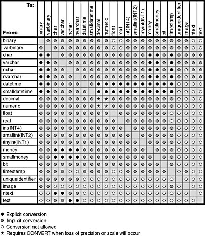
Table 9-10. Conversion table from the SQL Server documentation.
Table 9-11. Date and time functions in Transact-SQL.
| Date Function | Return Type | Description |
|---|---|---|
| DATEADD ( datepart , number , datetime ) | Datetime | Produces a date by adding an interval to a specified date. |
| DATEDIFF ( datepart , datetime1 , datetime2 ) | Int | Returns the number of datepart "boundaries" crossed between two specified dates. |
| DATENAME ( datepart , datetime ) | VarchaR | Returns a character string representing the specified datepart of the specified date. |
| DATEPART ( datepart , datetime ) | Int | Returns an integer representing the specified datepart of the specified date. |
| GETDATE() | Datetime | Returns the current system date and time in the SQL Server standard internal format for datetime values. |
Table 9-12. Values for the datepart parameter.
| datepart (Full Name) | Abbreviation | Values |
|---|---|---|
| year | Yy | 1753_9999 |
| quarter | 1_4 | |
| month | Mm | 1_12 |
| dayofyear | Dy | 1_366 |
| day | Dd | 1_31 |
| week | Wk | 1_53 |
| weekday | Dw | 1_7 (Sunday_Saturday) |
| hour | Hh | 0_23 |
| minute | Mi | 0_59 |
| second | Ss | 0_59 |
| millisecond | Ms | 0_999 |
As do other functions, the date functions provide more than simple convenience. Suppose that we needed to find all records entered on the second Tuesday of every month and all records entered within 48 weeks of today. Without SQL Server date functions, the only way we could accomplish such a query would be to select all the rows and return them to the application and then filter them there. With a lot of data and a slow network, this can get ugly. With the date functions, the process is simple and efficient, and only the rows that meet this criteria are selected. For this example, assume that the table records includes these columns:
Record_number int Entered_on datetime |
This query will return the desired rows:
SELECT Record_number, Entered_on FROM records WHERE DATEPART(WEEKDAY, Entered_on)=3 -- Tuesday is 3rd day of week (in USA) AND DATEPART(DAY, Entered_on) BETWEEN 8 AND 14 -- The 2nd week is from the 8th to 14th AND DATEDIFF(WEEK, Entered_on, GETDATE()) <= 48 -- Within 48 weeks of today |
NOTE
The day of the week considered "first" is locale-specific and depends on the DATEFIRST setting.
SQL Server 7 also allows you to add or subtract an integer to or from a datetime value. This is actually just a shortcut for the DATEADD function, with a datepart of Day. For example, the following two queries are equivalent. They'll each return the date 14 days from today:
select dateadd(day, 14, getdate()) select getdate() + 14 |
The date functions don't do any rounding. The DATEDIFF() function just subtracts the components from each date that correspond to the datepart specified. For example, to find the number of years between New Year's Day and New Year's Eve of the same year, this query would return a value of 0. Because the datepart is specifying years, SQL Server will subtract the year part of the two dates, and because they're the same, the result of subtracting them is 0:
select datediff(yy, 'Jan 1, 1998', 'Dec 31, 1998') |
However, if we wanted to find the difference in years between New Year's Eve of one year and New Year's Day (the next day), the following query would return a value of 1, because the difference in the year part is 1:
select datediff(yy, 'Dec 31, 1998', 'Jan 1, 1999') |
There's no built-in mechanism for determining whether two date values are actually the same day, unless you've forced all datetime values to use the default time of midnight. (We saw a technique for doing so earlier in this section.) If you want to compare two datetime values (@date1 and @date2) to determine whether they're on the same day, regardless of the time, one technique would be to use a three-part condition like this:
if (datepart(mm, @date1) = datepart(mm, @date2) and (datepart(dd, @date1) = datepart(dd, @date2) and (datepart(yy, @date1) = datepart(yy, @date2) print 'The dates are the same' |
Alternatively, we could use a trick. If two dates are really the same, they both occurred the same number of days after any other specific date. Because the DATEDIFF() function ignores the time when we use a datepart of Day, we could merely check to see whether DATEDIFF() returns the same value for the two dates. Note that we could use any date constant in this query, as long as we use the same one in both function calls:
if datediff(day, '1/1/99', @date1) = datediff(day, '1/1/99', @date2) print 'The dates are the same' |
Math Functions
Transact-SQL math functions are straightforward and typical. Many are specialized and of the type you learned about in trigonometry class. (If you don't have an engineering or mathematical application, you probably won't use those.) A handful of math functions are useful in general types of queries in applica- tions that aren't mathematical in nature. ABS(), CEILING(), FLOOR(), and ROUND() are most useful functions for general queries to find values within a certain range.
The random number function, RAND(), is useful to generate test data or conditions. (We'll see examples of RAND() in Chapter 12.)
Table 9-13 shows the complete list of math functions and a few simple examples. (Some of the examples use other functions in addition to the math ones to illustrate how to use functions within functions.)
Table 9-13. Math functions in Transact-SQL.
| Function | Parameters | Result |
|---|---|---|
| ABS | ( numeric_expr ) | Absolute value of the numeric expression. Results returned are of the same type as numeric_expr . |
| ACOS | ( float_expr ) | Angle (in radians) whose cosine is the specified approximate numeric ( float ) expression. |
| ASIN | ( float_expr ) | Angle (in radians) whose sine is the specified approximate numeric ( float ) expression. |
| ATAN | ( float_expr ) | Angle (in radians) whose tangent is the specified approximate numeric ( float ) expression. |
| ATN2 | ( float_expr1 , float_expr2 ) | Angle (in radians) whose tangent is ( float_expr1/float_expr2 ) between two approximate numeric ( float ) expressions. |
| CEILING | ( numeric_expr ) | Smallest integer greater than or equal to the numeric expression. Result returned is the integer portion of the same type as numeric_expr . |
| COS | ( float_expr ) | Trigonometric cosine of the specified angle (in radians) in an approximate numeric ( float ) expression. |
| COT | ( float_expr ) | Trigonometric cotangent of the specified angle (in radians) in an approximate numeric ( float ) expression. |
| DEGREES | ( numeric_expr ) | Degrees converted from radians of the numeric expression. Results are of the same type as numeric_expr . |
| EXP | ( float_expr ) | Exponential value of the specified approximate numeric ( float ) expression. |
| FLOOR | ( numeric_expr ) | Largest integer less than or equal to the specified numeric expression. Result is the integer portion of the same type as numeric_expr . |
| LOG | ( float_expr ) | Natural logarithm of the specified approximate numeric ( float ) expression. |
| LOG10 | ( float_expr ) | Base-10 logarithm of the specified approximate numeric ( float ) expression. |
| PI | () | Constant value of 3.141592653589793. |
| POWER | ( numeric_expr , y ) | Value of numeric expression to the power of y , where y is a numeric datatype ( decimal, float, int, money, numeric, real, smallint, smallmoney, or tinyint ). Result is of the same type as numeric_expr . |
| RADIANS | ( numeric_expr ) | Radians converted from degrees of the numeric expression. Result is of the same type as numeric_expr . |
| RAND | ([ seed ]) | Random approximate numeric ( float ) value between 0 and 1, optionally specifying an integer expression as the seed. |
| ROUND | ( numeric_expr , length ) | Numeric expression rounded off to the length (or precision) specified as an integer expression ( tinyint, smallint, or int ). Result is of the same type as numeric_expr . ROUND() always returns a value even if length is illegal. If the specified length is positive and longer than the digits after the decimal point, 0 is added after the fraction dig- its. If the length is negative and larger than or equal to the digits before the decimal point, ROUND() returns 0.00. |
| SIGN | ( numeric_expr ) | Returns the positive (+1), zero (0), or negative (_1) sign of the numeric expression. Result is of the same type as numeric_expr . |
| SIN | ( float_expr ) | Trigonometric sine of the specified angle (measured in radians) in an approximate numeric ( float ) expression. |
| SQRT | ( float_expr ) | Square root of the specified approximate numeric ( float ) expression. |
| SQUARE | ( float_expr ) | Square of the specified approximate numeric ( float ) expression. |
| TAN | ( float_expr ) | Trigonometric tangent of the specified angle (measured in radians) in an approximate numeric ( float ) expression. |
The following examples show some of the math functions at work:
EXAMPLE 1
Produce a table with the cosine, sine, and tangent of all angles in multiples of 10 from 0 through 180. Format the return value as a string of six characters, with the value rounded to four decimal places.
DECLARE @degrees smallint DECLARE @radians float SELECT @degrees=0 SELECT @radians=0 WHILE (@degrees <= 180) BEGIN SELECT DEGREES=@degrees, RADIANS=STR(@radians, 7, 5), SINE=STR(SIN(@radians), 7, 5), COSINE=STR(COS(@radians), 7, 5), TANGENT=STR(TAN(@radians), 7, 5) SELECT @degrees=@degrees + 10 SELECT @radians=RADIANS(CONVERT(float, @degrees)) END |
NOTE
This example actually produces 19 different result sets because the SELECT statement is issued once for each iteration of the loop. These separate result statements are concatenated and appear as one result set in this example. That works fine for illustrative purposes, but you should avoid doing an operation like this in the real world, especially on a slow network. Every one of the result sets carries with it metadata to describe itself to the client application. Chapter 12 shows a better technique.
And here are the results concatenated as a single table:
DEGREES RADIANS SINE COSINE TANGENT ------- ------- ------- ------- ------- 0 0.0000 0.0000 1.0000 0.0000 10 0.1745 0.1736 0.9848 0.1763 20 0.3491 0.3420 0.9397 0.3640 30 0.5236 0.5000 0.8660 0.5774 40 0.6981 0.6428 0.7660 0.8391 50 0.8727 0.7660 0.6428 1.1918 60 1.0472 0.8660 0.5000 1.7321 70 1.2217 0.9397 0.3420 2.7475 80 1.3963 0.9848 0.1736 5.6713 90 1.5708 1.0000 0.0000 ******* 100 1.7453 0.9848 -0.1736 -5.6713 110 1.9199 0.9397 -0.3420 -2.7475 120 2.0944 0.8660 -0.5000 -1.7321 130 2.2689 0.7660 -0.6428 -1.1918 140 2.4435 0.6428 -0.7660 -0.8391 150 2.6180 0.5000 -0.8660 -0.5774 160 2.7925 0.3420 -0.9397 -0.3640 170 2.9671 0.1736 -0.9848 -0.1763 180 3.1416 0.0000 -1.0000 -0.0000 |
EXAMPLE 2
Express in whole-dollar terms the range of prices (non-null) of all books in the titles table. This example combines the scalar functions FLOOR() and CEILING() inside the aggregate functions MIN() and MAX():
SELECT 'Low End'=MIN(FLOOR(price)), 'High End'=MAX(CEILING(price)) FROM titles |
And the result:
Low End High End ------- -------- 2.00 23.00 |
EXAMPLE 3
Use the same records table that was used earlier in the date functions example. Find all records within 150 days of September 30, 1997. Without the absolute value function ABS(), you would have to use BETWEEN or to provide two search conditions and OR them to account for both 150 days earlier and 150 days later than that date. ABS() lets you easily reduce that to a single search condition.
SELECT Record_number, Entered_on FROM records WHERE ABS(DATEDIFF(DAY, Entered_on, '1997.09.30')) <= 150 -- Plus or minus 150 days |
String Functions
String functions make it easier to work with character data. They let you slice and dice character data, search it, format it, and alter it. Like other scalar functions, string functions allow you to perform functions directly in your search conditions and SQL batches that would otherwise need to be returned to the calling application for further processing. (Also, remember the concatenation operator, +, for concatenating strings. You'll use this operator often in conjunction with the string functions.)
The string functions appear in Table 9-14. For more detailed information, consult the online documentation.
Table 9-14. String functions in Transact-SQL.
| Function | Parameters | Returns |
|---|---|---|
| ASCII | ( char_expr ) | Indicates the numeric code value of the leftmost character of a character expression. |
| CHAR | ( integer_expr ) | Character represented by the ASCII code. The ASCII code should be a value from 0 through 255; otherwise, NULL is returned. |
| CHARINDEX | (' pattern ', expression ) | Returns the starting position of the specified exact pattern. A pattern is a char_expr . The second parameter is an expression, usually a column name, in which SQL Server searches for pattern . |
| DIFFERENCE | ( char_expr1 , char_expr2 ) | Shows the difference between the values of two character expressions as returned by the SOUNDEX function. DIFFERENCE compares two strings and evaluates the similarity between them, returning a value 0 through 4. The value 4 is the best match. |
| LEFT | ( char_expression , int_expression ) | Returns int_expression characters from the left of the char_expression. |
| LEN | ( char_expression ) | Returns the number of characters, rather than the number of bytes, of char_expression , excluding trailing blanks. |
| LOWER | ( char_expr ) | Converts uppercase character data to lowercase. |
| LTRIM | ( char_expr ) | Removes leading blanks. |
| NCHAR | ( int_expression ) | Returns the Unicode character with code int_expression , as defined by the Unicode standard. |
| PATINDEX | ('% pattern %', expression ) | Returns the starting position of the first occurrence of pattern in the specified expression, or 0 if the pattern isn't found. |
| QUOTENAME | QUOTENAME (' char_string '[,' quote_character ']) | Returns a Unicode string with quote_character used as the delimiter to make the input string a valid SQL Server delimited identifier. |
| REPLACE | (' char_expression1 ', ' char_expression2 ', ' char_expression3 ') | Replaces all occurrences of char_expression2 in char_expression1 with char_expression3 . |
| REPLICATE | ( char_expr , integer_expr ) | Repeats a character expression a specified number of times. If integer_expr is negative, NULL is returned. |
| REVERSE | ( char_expr ) | Returns the char_expr backwards . This function takes a constant, variable, or column as its parameter. |
| RIGHT | ( char_expr , integer_expr ) | Part of a character string starting integer_expr characters from the right. If integer_expr is negative, NULL is returned. |
| RTRIM | ( char_expr ) | Removes trailing blanks. |
| SOUNDEX | ( char_expr ) | Returns a four-character (SOUNDEX) of two strings. The SOUNDEX function converts an alpha string to a four-digit code used to find similar-sounding words or names. |
| SPACE | ( integer_expr ) | Returns a string of repeated spaces. The number of spaces is equal to integer_expr . If integer_expr is negative, NULL is returned. |
| STR | ( float_expr [, length [, decimal ]]) | Returns character data converted from numeric data. The length is the total length, including decimal point, sign, digits, and spaces. The decimal value is the number of spaces to the right of the decimal point. |
| STUFF | ( char_expr1 , start , length , char_expr2 ) | Deletes length characters from char_expr1 at start and then inserts char_expr2 into char_expr1 at start . |
| SUBSTRING | ( expression , start , length ) | Returns part of a character or binary string. The first parameter can be a character or binary string, a column name, or an expression that includes a column name. The second parameter specifies where the substring begins. The third parameter specifies the number of characters in the substring. |
| UNICODE | (' nchar_expression ') | Returns the integer value, as defined by the Unicode standard, for the first character of nchar_expression . |
| UPPER | ( char_expr ) | Converts lowercase character data to uppercase. |
ASCII() and CHAR() functions The function name ASCII() is really a bit of a misnomer. ASCII is only a 7-bit character set and hence can deal with only 128 characters. The character parameter to this function doesn't need to be an ASCII character. The ASCII function returns the code point for the character set installed with SQL Server, so the return value can be from 0 through 255. For example, if SQL Server is installed with the ISO 8859-1 (Latin-1) character set, the statement
SELECT ASCII('') |
returns 196. (The character isn't an ASCII character.)
The CHAR() function is handy for generating test data, especially when combined with RAND() and REPLICATE(). (We'll see an example in Chapter 12.) CHAR() is also commonly used for inserting control characters such as tabs and carriage returns into your character string. Suppose, for example, that we want to return authors' last names and first names concatenated as a single field, but with a carriage return (0x0D, or decimal 13) separating them so that without further manipulation in our application, the names occupy two lines when displayed. The CHAR() function makes this simple:
SELECT 'NAME'=au_fname + CHAR(13) + au_lname FROM authors |
Here's the abbreviated result:
NAME -------- Johnson White Marjorie Green Cheryl Carson Michael O'Leary Dean Straight Meander Smith Abraham Bennet Ann Dull |
UPPER() and LOWER() functions The UPPER() and LOWER() functions are useful if you must perform case-insensitive searches on a server that is case-sensitive. On a case-sensitive server, for example, this query finds no rows even though author name Cheryl Carson is included in that table:
SELECT COUNT(*) FROM authors WHERE au_lname='CARSON' |
If we change the query to the following, the row will be found:
SELECT COUNT(*) FROM authors WHERE UPPER(au_lname)='CARSON' |
If the value to be searched might be of mixed case, you need to use the function on both sides of the equation. This query would find the row on the case-sensitive server:
DECLARE @name_param varchar(30) SELECT @name_param='cArSoN' SELECT COUNT(*) FROM authors WHERE UPPER(au_lname)=UPPER(@name_param) |
In these examples, even though we might have an index on au_lname, it won't be useful because the index keys aren't uppercase. (However, it would be possible to use triggers to maintain an uppercase copy of the column, index it, and then use it for searching.)
You'll also often want to use UPPER() or LOWER() in stored procedures in which character parameters are used. For example, in a procedure that expects Y or N as a parameter, you'll likely want to use one of these functions in case y is entered instead of Y .
TRIM functions The functions LTRIM() and RTRIM() are handy for dealing with leading or trailing blanks. Recall that by default (and if you don't enable the ANSI_PADDING setting), a varchar datatype is automatically right- trimmed of blanks, but a fixed-length char isn't. Suppose that we want to concatenate the type column and the title_id column from the titles table, with a colon separating them but with no blanks. The following query doesn't work because the trailing blanks are retained from the type column:
SELECT type + ':' + title_id FROM titles |
This returns (in part):
------------------- business :BU1032 business :BU1111 business :BU2075 business :BU7832 mod_cook :MC2222 mod_cook :MC3021 UNDECIDED :MC3026 popular_comp:PC1035 popular_comp:PC8888 popular_comp:PC9999 |
But RTRIM() returns what we want:
SELECT RTRIM(type) + ':' + title_id FROM titles |
And the result (in part):
------------------- business:BU1032 business:BU1111 business:BU2075 business:BU7832 mod_cook:MC2222 mod_cook:MC3021 UNDECIDED:MC3026 popular_comp:PC1035 popular_comp:PC8888 popular_comp:PC9999 |
String manipulation functions Functions are useful for searching and manipulating partial strings that include SUBSTRING(), CHARINDEX(), PATINDEX(), STUFF(), REPLACE(), REVERSE(), and REPLICATE(). CHARINDEX() and PATINDEX() are similar, but CHARINDEX() demands an exact match, and PATINDEX() works with a regular expression search.
NOTE
You could use one or both of these functions as a replace-ment for LIKE as well. For example, instead of saying WHERE name LIKE '%SMITH%' , you could say WHERE CHARINDEX('Smith', name) > 0 . Before SQL Server version 6.0, the CHARINDEX() formulation above was much faster than LIKE for an exact pattern match query such as this. But this is no longer true ”they're equal in performance.
Suppose we want to change occurrences of the word "computer" within the notes field of the titles table and replace it with "Hi-Tech-Computers." Assume that SQL Server is case-sensitive and, for simplicity, that we know that "computer" won't appear more than once per column. We want to be careful that the word "computers," which is already plural, isn't also changed. We can't just rely on searching on "computer" with a trailing blank, because the word might fall at the end of the sentence followed by a period or a comma. The regular expression computer[^s] always finds the word "computer" and ignores "computers," so it'll work perfectly with PATINDEX().
Here's the data before the change:
SELECT title_id, notes FROM titles WHERE notes LIKE '%[Cc]omputer%' title_id notes -------- ------------------------------------------------------ BU7832 Annotated analysis of what computers can do for you: a no-hype guide for the critical user. PC8888 Muckraking reporting on the world's largest computer hardware and software manufacturers. PC9999 A must-read for computer conferencing. PS1372 A must for the specialist, this book examines the difference between those who hate and fear computers and those who don't. PS7777 Protecting yourself and your loved ones from undue emotional stress in the modern world. Use of computer and nutritional aids emphasized. |
You might consider using the REPLACE() function to make the substitution. However, REPLACE() requires that we search for a specific string that can't include wildcards like [^s]. Instead, we can use the older STUFF() function, which has a slightly more complex syntax. STUFF() requires that we specify the starting location within the string to make a substitution. We can use PATINDEX() to find the correct starting location, and PATINDEX() allows wildcards:
UPDATE titles SET notes=STUFF(notes, PATINDEX('%computer[^s]%', notes), DATALENGTH('computer'), 'Hi-Tech-Computers') WHERE PATINDEX('%computer[^s]%', notes) > 0 |
Here's the data after the change:
SELECT title_id, notes FROM titles WHERE notes LIKE '%[Cc]omputer%' title_id notes -------- ------------------------------------------------------ BU7832 Annotated analysis of what computers can do for you: a no-hype guide for the critical user. PC8888 Muckraking reporting on the world's largest Hi-Tech- Computers hardware and software manufacturers. PC9999 A must-read for Hi-Tech-Computers conferencing. PS1372 A must for the specialist, this book examines the difference between those who hate and fear computers and those who don't. PS7777 Protecting yourself and your loved ones from undue emotional stress in the modern world. Use of Hi-Tech- Computers and nutritional aids emphasized. |
Of course, we could have simply provided 8 as the length parameter of the string "computer" to be replaced. But we used yet another function, DATALENGTH(), which would be more realistic if we were creating a general-purpose, search-and-replace procedure. Note that DATALENGTH() returns NULL if the expression is NULL, so in your applications, you might go one step further and use DATALENGTH() inside the ISNULL() function to return 0 in the case of NULL.
The REPLICATE() function is useful for adding filler characters ”such as for test data. (In fact, generating test data seems to be about the only practical use for this function.) The SPACE() function is a special-purpose version of REPLICATE(): it's identical to using REPLICATE with the space character. REVERSE() reverses a character string (a standard programming puzzle, for sure, but not too common in production applications). REVERSE() can be used in a few cases to store and, more importantly, to index a character column backward to get more selectivity from the index. But in general, these three functions are rarely used.
SOUNDEX() and DIFFERENCE() Functions
If you've ever wondered how telephone operators are able to give you telephone numbers so quickly when you call directory assistance, chances are they're using a SOUNDEX algorithm. The SOUNDEX() and DIFFERENCE() functions let you search on character strings that sound similar when spoken. SOUNDEX() converts each string to a four-character code. DIFFERENCE() can then be used to evaluate the level of similarity between the SOUNDEX values for two strings as returned by SOUNDEX(). For example, you could use these functions if you wanted to look at all rows that sound like "Erickson," and they would find "Erickson," "Erikson," "Ericson," "Ericksen," "Ericsen," and so on.
SOUNDEX algorithms are commonplace in the database business, but the exact implementation can vary from vendor to vendor. For SQL Server's SOUNDEX() function, the first character of the four-character SOUNDEX code is the first letter of the word, and the remaining three characters are single digits that describe the phonetic value of the first three consonants of the word with the underlying assumption that there's one consonant per syllable. Identical consonants right next to each other are treated as a single consonant. Only nine phonetic values are possible in this scheme, because only nine possible digits exist. SOUNDEX() relies on phonetic similarities between sounds to group consonants together. In fact, SQL Server's SOUNDEX() algorithm uses only seven of the possible nine digits. No SOUNDEX() code uses the digits 8 or 9.
Vowels are ignored, as are the characters "h" and "y," so "Zastrak" would have the same code as "Zasituryk." If no second or subsequent consonant exists, the phonetic value for it is 0. In addition, SQL Server's SOUNDEX() algorithm stops evaluating the string as soon as the first nonalphabetic character is found. So if you have a hyphenated or two-word name (with a space in between), SOUNDEX() will ignore the second part of the name. More seriously, SOUNDEX() stops processing names as soon as it finds an apostrophe. So "O'Flaherty", "O'Leary", and "O'Hara" all have the same SOUNDEX() code, namely O000.
DIFFERENCE() internally compares two SOUNDEX values and returns a score from 0 through 4 to indicate how close the match is. A score of 4 is the best match, and 0 means no matches were found. Executing DIFFERENCE(a1, a2) first generates the four-character SOUNDEX values for a1 (call it sx_a1 ) and a2 (call it sx_a2 ). Then if all four values of the SOUNDEX value sx_a2 match the values of sx_a1 , the match is perfect, and the level is 4. Note that this compares the SOUNDEX values by character position, not by actual characters.
For example, the names "Smythe" and "Smith" both have a SOUNDEX() value of S530, so their difference level is 4, even though the spellings differ . If the first character (a letter, not a number) of the SOUNDEX value sx_a1 is the same as the first character of sx_a2 , the starting level is 1. If the first character is different, the starting level is 0. Then each character in sx_a2 is successively compared to all characters in sx_a1 . When a match is found, the level is incremented and the next scan on sx_a1 starts from the location of the match. If no match is found, the next sx_a2 character is compared to the entire four-character list of sx_a1 .
The above description of the algorithms should make it clear that SOUNDEX() at best provides an approximation . Even so, sometimes it works extremely well. Suppose we want to query the authors table for names that sound similar to "Larsen." We'll define similar to mean "have a SOUNDEX() value of 3 or 4":
SELECT au_lname, Soundex=SOUNDEX(au_lname), Diff_Larsen=DIFFERENCE(au_lname, 'Larson') FROM authors WHERE DIFFERENCE(au_lname, 'Larson') >= 3 |
Here's the result:
au_lname Soundex Diff_Larsen -------- ------- ----------- Carson C625 3 Karsen K625 3 |
In this case, we found two names that rhyme with "Larsen" and didn't get any bad hits of names that don't seem close. Sometimes you'll get odd results, but if you follow the algorithms above, you'll understand how these oddities occur. For example, do you think "Bennet" and "Smith" sound similar? Well, SOUNDEX() does. When you investigate, you can see why the two names have a similar SOUNDEX() value. The SOUNDEX values have a different first letter, but the m and n sounds are converted to the same digit, and both names include a t, which is converted to a digit for the third position. "Bennet" has nothing to put in the fourth position, so it gets a 0. For Smith, the h becomes a 0. So, except for the initial letter, the rest of the SOUNDEX() strings are the same. Hence, the match.
This type of situation happens often with SOUNDEX() ”you'll get hits on values that don't seem close, although usually you won't miss the ones that are similar. So if you query the authors table for similar values (with a DIFFERENCE() value of 3 or 4) as "Smythe," you get a perfect hit on "Smith" as you'd expect, but you also get a close match for "Bennet," which is far from obvious:
SELECT au_lname, Soundex=SOUNDEX(au_lname), Diff_Smythe=DIFFERENCE(au_lname, 'Smythe') FROM authors WHERE DIFFERENCE(au_lname, 'Smythe') >= 3 au_lname Soundex Diff_Smythe -------- ------- ----------- Smith S530 4 Bennet B530 3 |
Sometimes SOUNDEX() misses close matches altogether. This happens when consonant blends are present. For example, you might expect to get a close match between "Knight" and "Nite." But you'll get a low value of 1 in the DIFFERENCE() between the two:
SELECT "SX_KNIGHT"=SOUNDEX('Knight'), "SX_NITE"=SOUNDEX('Nite'), "DIFFERENCE"=DIFFERENCE('Nite', 'Knight') SX_KNIGHT SX_NITE DIFFERENCE --------- ------- ---------- K523 N300 1 |
System Functions
System functions are most useful for returning certain metadata or configuration settings. Table 9-15 lists of some of the more commonly used system functions, and it's followed by a brief discussion of the interesting features of a few of them. For complete details, see the SQL Server online documentation.
Table 9-15. Some commonly used system functions.
| Function | Parameters | Returns |
|---|---|---|
| APP_NAME | NONE | Returns the program name for the current connection if one has been set by the program before logging on. |
| COALESCE | ( expression1 , expression2 , ... expressionN ) | A specialized form of the CASE statement. Returns the first non-null expression. |
| COL_LENGTH | (' table_name ', ' column _ name ') | The defined (maximum) storage length of a column. |
| COL_NAME | ( table _ id , column _ id ) | The name of the column. |
| DATALENGTH | (' expression ') | The length of an expression of any datatype. |
| DB_ID | ([' database_name ']) | The database identification number. |
| DB_NAME | ([ database _ id ]) | The database name. |
| GETANSINULL | ([' database_name ']) | The default nullability for the database. Returns 1 when the nullability is the ANSI NULL default. |
| HOST_ID | NONE | The workstation identification number. |
| HOST_NAME | NONE | The workstation name. |
| IDENT_INCR | (' table_or_view ') | The increment value specified during creation of an identity column of a table or view that includes an identity column. |
| IDENT_SEED | (' table_or_view ') | The seed value specified during creation of an identity column of a table or view that includes an identity column. |
| INDEX_COL | (' table _ name ', index _ id , key_id ) | The indexed column name(s). |
| ISDATE | ( expression _ of_possible_date ) | Checks whether an expression is a datetime datatype or a string in a recognizable datetime format. Returns 1 when the expression is compatible with the datetime type; otherwise, returns 0. |
| ISNUMERIC | ( expression _ of _ possible _ number ) | Checks whether an expression is a numeric datatype or a string in a recognizable number format. Returns 1 when the expression is compatible with arithmetic operations; otherwise, returns 0. |
| ISNULL | ( expression , value ) | Replaces NULL entries with the specified value. |
| NULLIF | ( expression1 , expression2 ) | A specialized form of CASE. The resulting expression is NULL when expression1 is equivalent to expression2 . |
| OBJECT_ID | (' object_name ') | The database object identification number. |
| OBJECT_NAME | ( object_id ) | The database object name. |
| STATS_DATE | ( table_id , index_id ) | The date when the statistics for the specified index ( index_id ) were last updated. |
| SUSER_ID | ([' login_name ']) | The user's login ID number. |
| SUSER_NAME | ([ server_user_id ]) | The user's login name. |
| SUSER_SID | ([' login_name ']) | The security identification number (SID) for the user's login name. |
| SUSER_SNAME | ([ server_user_sid ]) | The login identification name from a user's security identification number (SID). |
| USER_ID | ([' user_name ']) | The user's database ID number. |
| USER_NAME | ([ user_id ]) | The user's database username. |
The DATALENGTH() function is most often used with variable-length data, especially character strings, and it tells you the actual storage length of the expression (typically a column name). A fixed-length datatype always returns the storage size of its defined type (which is also its actual storage size), which makes it identical to COL_LENGTH() for such a column. The DATALENGTH() of any NULL expression returns NULL. The OBJECT_ID(), OBJECT_NAME(), SUSER_ID(), SUSER_NAME() SUSER_SAME(), SUSER_SID(), USER_ID(), USER_NAME(), COL_NAME(), DB_ID(), and DB_NAME() functions are commonly used to more easily eliminate the need for joins between system catalogs and to get run-time information dynamically.
For example, recognizing that an object name is unique within a database for a specific user, we can use the statement on the next page to determine whether an object by the name "foo" exists for our current user ID; if so, we can drop it ( assuming that we know it's a table).
IF (SELECT id FROM sysobjects WHERE id=OBJECT_ID('foo') AND uid=USER_ID() AND type='U') > 0 DROP TABLE foo |
System functions can be handy with constraints and views. Recall that a view can benefit from the use of system functions. For example, if the accounts table includes a column that is the system login ID of the user to whom the account belongs, we can create a view of the table that allows the user to work only with his or her own accounts. We do this simply by making the WHERE clause of the view something like this:
WHERE system_login_id=SUSER_SID() |
Or if we want to ensure that updates on a table occur only from an ap-plication named CS_UPDATE.EXE, we can use a CHECK constraint in the following way:
CONSTRAINT APP_CHECK (APP_NAME()='CS_UPDATE.EXE') |
For this particular example, the check is by no means foolproof, as the application must set the app_name in its login record. A rogue application could simply lie. To prevent casual use by someone running an application like isql.exe, the above formulation might be just fine for your needs. But if you're worried about hackers, this formulation isn't appropriate. Other functions, such as SUSER_SID(), have no analogous way to be explicitly set, so they're better for security operations like this.
The ISDATE() and ISNUMERIC() functions can be useful to determine whether data is appropriate for an operation. For example, suppose that your predecessor didn't know much about using a relational database and defined a column as type char and then stored values in it that were naturally of type money . Then your predecessor compounded the problem by sometimes encoding letter codes in the same field as notes. You're trying to work with the data as is (eventually you'll clean it up, but you have a deadline to meet), and you need to get a sum and average of all the values, whenever a value that makes sense to use is present. (If you think this example is contrived, talk to a programmer in an MIS shop of a Fortune 1000 company with legacy applications and ask whether this situation sounds uncommon.) Suppose that the table has a varchar(20) column named acct_bal with these values:
acct_bal -------- 205.45 E (NULL) B 605.78 32.45 8 98.45 64.23 8456.3 |
If you try to simply use the aggregate functions directly, you'll get error 409:
SELECT SUM(acct_bal), AVG(acct_bal) FROM bad_column_for_money Msg 409, Level 16, State 2 The sum or average aggregate operation cannot take a varchar data type as an argument. |
If you try to use CONVERT(), the columns that contain alphabetic characters will cause the CONVERT() to fail:
SELECT "SUM"=SUM(CONVERT(money, acct_bal)), "AVG"=AVG(CONVERT(money, acct_bal)) FROM bad_column_for_money Msg 235, Level 16, State 0 Cannot convert CHAR value to MONEY. The CHAR value has incorrect syntax. |
But if you use both CONVERT() in the select list and ISNUMERIC() in the WHERE clause to choose only those values for which a conversion would be possible, everything works great:
SELECT "SUM"=SUM(CONVERT(money, acct_bal)), "AVG"=AVG(CONVERT(money, acct_bal)) FROM bad_column_for_money WHERE ISNUMERIC(acct_bal)=1 SUM AVG -------- -------- 9,470.66 1,352.95 |
Property Functions
You can think of property functions as a type of system function because they allow you access to metadata. In earlier versions of SQL Server, the only way to determine which options or properties an object had was to actually query a system table, and possibly even decode a bitmap status column. SQL Server 7 provides a set of functions that return information about databases, files, filegroups, indexes, objects, and datatypes.
For example, to determine whether a database has the select into/bulkcopy property set, we can use the DATABASEPROPERTY() function:
IF DATABASEPROPERTY('pubs', 'IsBulkCopy') = 1 /* call a procedure than runs the BULK INSERT command */ else /* call a procedure that does something else */ |
Many of the properties that we can check for correspond to database options that can be set with the sp_dboption stored procedure. One example is the select into/bulkcopy option, which determines the value of the IsBulkCopy property. Other properties, such as IsInLoad, are set internally by SQL Server. For a complete list of all the possible database properties and their possible values, please see the SQL Server documentation. Also in the documentation, you'll find the complete list of properties and possible values for use with the following functions:
- COLUMNPROPERTY()
- FILEGROUPPROPERTY()
- FILEPROPERTY()
- INDEXPROPERTY()
- OBJECTPROPERTY()
- TYPEPROPERTY()
Niladic Functions
ANSI SQL-92 has a handful of what it calls niladic functions ”a fancy way to indicate that these functions don't accept any parameters. Niladic functions were implemented for version 6.0 and map directly to one of SQL Server's system functions. Frankly, they were added to SQL Server 6.0 because they were mandated for conformance to the ANSI SQL-92 standard ”all of their functionality was already provided. Table 9-16 on the following page shows niladic functions and their equivalent SQL Server system functions.
Table 9-16. Niladic functions and equivalent SQL Server functions.
| Niladic Function | Equivalent SQL Server System Function |
|---|---|
| CURRENT_TIMESTAMP | GETDATE() |
| SYSTEM_USER | SUSER_NAME() |
| CURRENT_USER | USER_NAME() |
| SESSION_USER | USER_NAME() |
| USER | USER_NAME() |
If you execute the following two SELECT statements, you'll see that they return identical results:
SELECT CURRENT_TIMESTAMP, USER, SYSTEM_USER, CURRENT_USER, SESSION_USER SELECT GETDATE(), USER_NAME(), SUSER_NAME(), USER_NAME(), USER_NAME() |
Other Parameterless Functions
As mentioned earlier in the chapter, the older SQL Server documentation refers to a set of parameterless system functions as global variables, because they're designated by @@ , which is similar to the designation for local variables. However, these values aren't variables, because you can't declare them and you can't assign them values.
These functions are global only in the sense that any connection can access their values. However, in many cases the value returned by these functions is specific to the connection. For example, @@ERROR represents the last error number generated for a specific connection, not the last error number in the entire system. @@ROWCOUNT represents the number of rows selected or affected by the last statement for the current connection.
Many of these parameterless system functions keep track of performance-monitoring information for your SQL Server. These include @@CPU_BUSY, @@IO_BUSY, @@PACK_SENT, and @@PACK_RECEIVED.
Some of these functions are extremely static, and others are extremely volatile. For example, @@version represents the build number and code freeze date of the SQL Server executable ( sqlservr .exe) that you're running. It will change only when you upgrade or apply a service pack. Functions like @@ROWCOUNT are extremely volatile. Take a look at the code on the next page and its results.
select * from publishers select @@ROWCOUNT select @@ROWCOUNT |
And the results:
pub_id pub_name city state country ------ ------------------------- -------------------- ----- ---------- 0736 New Moon Books Boston MA USA 0877 Binnet & Hardley Washington DC USA 1389 Algodata Infosystems Berkeley CA USA 1622 Five Lakes Publishing Chicago IL USA 1756 Ramona Publishers Dallas TX USA 9901 GGG&G Mnchen NULL Germany 9952 Scootney Books New York NY USA 9999 Lucerne Publishing Paris NULL France (8 row(s) affected) ----------- 8 (1 row(s) affected) ----------- 1 (1 row(s) affected) |
Note that the first time @@ROWCOUNT was selected, it returned the number of rows in the publishers table (8). The second time @@ROWCOUNT was selected, it returned the number of rows returned by the previous select @@ROWCOUNT (1). Any query you execute that affects rows will change the value of @@ROWCOUNT.
SEE ALSO
For the complete list of parameterless functions, refer to the SQL Server documentation. You can access the full set of documentation from the startup menu of the SQL Server evaluation CD (included with this book). You don't have to actually install SQL Server to read the documentation on the CD.
EAN: 2147483647
Pages: 144
- Chapter I e-Search: A Conceptual Framework of Online Consumer Behavior
- Chapter IV How Consumers Think About Interactive Aspects of Web Advertising
- Chapter VII Objective and Perceived Complexity and Their Impacts on Internet Communication
- Chapter XIV Product Catalog and Shopping Cart Effective Design
- Chapter XVI Turning Web Surfers into Loyal Customers: Cognitive Lock-In Through Interface Design and Web Site Usability