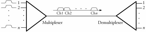
Section 3.1. Multiplexers

3.1. Multiplexers

Multiplexers are used in a network for maximum transmission capacity of a high-bandwidth line. Regardless of the type of multiplexer, multiplexing is a technique that allows many communication sources to transmit data over a single physical line. Multiplexing schemes can be divided into three basic categories: frequency-division multiplexing , wavelength-division multiplexing , and time-division multiplexing .

3.1.1. Frequency-Division Multiplexing (FDM)

In frequency-division multiplexing (FDM), the frequency spectrum is divided into frequency bands, or channels , in which each user can be assigned a band . Figure 3.1 shows how n frequency channels are multiplexed using FDM. When many channels are multiplexed together, a certain guard band is allocated to keep the channels well separated.

Figure 3.1. A frequency-division multiplexer (FDM) with n inputs

To implement a multiplexer, the original frequencies at any of n inputs of the multiplexer are raised, each by a different constant amount. Then, the n new frequency bands are combined to let no two channels occupy the same portion of the spectrum. Despite the guard bands between the channels, any two adjacent channels have some overlap because channel spectra do not have sharp edges. This overlap normally creates spike noise at the edge of each channel. FDM is normally used over copper wires or microwave channels and is suitable for analog circuitry .

3.1.2. Wavelength-Division Multiplexing (WDM)

Wavelength-division multiplexing (WDM) is fundamentally the same as FDM, as depicted in Figure 3.2. WDM was invented as a variation of frequency-division multiplexing and is basically a multiplexing method of different wavelengths instead of frequencies. In the figure, n optical fibers come together at an optical multiplexer, each with its energy present at a different wavelength. The n optic lines are combined onto a single shared link for transmission to a distant destination. At the demultiplexer , each frame, including n channels, is split up over as many optical fibers as there were on the input side. At each output of the demultiplexer, a tuned filter refines the desired signal at the tuned wavelength, and thus all other wavelengths are bypassed.

Figure 3.2. A wavelength-division multiplexer (WDM) with n inputs

The main issue of WDM compared with FDM is that an optical system using a diffraction grating is completely passive and thus highly reliable. With higher-speed variations of WDM, the number of channels is very large, and the wavelengths are as close as 0.1 nm. Such systems are referred to as DWDM (dense WDM). Chapter 14 presents much more detail about WDM and its applications.

Example.	Consider a practical multiplexing system with 100 channels, each at rate 10 Gb/s. Compute the number of full-length movies per second that can be transferred with this WDM system.
Solution.	The total bit rate of this WDM is 100 x 10, or 1,000 Gb/s. Since a movie (MPEG-2 technology) requires 32 Gb/s bandwidth, the system can carry approximately 34 full-length movies per second.

3.1.3. Time-Division Multiplexing

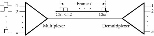
With a time-division multiplexing (TDM), users take turns in a predefined fashion, each one periodically getting the entire bandwidth for a portion of the total scanning time. Given n inputs, time is divided into frames , and each frame is further subdivided into time slots, or channels. Each channel is allocated to one input. (See Figure 3.3.) This type of multiplexing can be used only for digital data. Packets arrive on n lines, and the multiplexer scans them, forming a frame with n channels on its outgoing link. In practice, packet size is variable. Thus, to multiplex variable- sized packets, additional hardware is needed for efficient scanning and synchronization. TDM can be either synchronous or statistical .

Figure 3.3. A time-division multiplexer with n inputs

Synchronous TDM

In synchronous TDM, the multiplexer scans all lines without exception. The scanning time for each line is preallocated; as long as this time for a particular line is not altered by the system control, the scanner should stay on that line, whether or not there is data for scanning within that time slot. Therefore, a synchronous multiplexer does not operate efficiently , though its complexity stays low.

Once a synchronous multiplexer is programmed to produce same-sized frames, the lack of data in any channel potentially creates changes to average bit rate on the ongoing link. In addition to this issue, the bit rates of analog and digital data being combined in a multiplexer sometimes need to be synchronized. In such cases, dummy pulses can be added to an input line with bit rate shortcoming. This technique of bit-rate synchronization is called pulse stuffing .

Example.

Consider the integration of three analog sources and four identical digital sources through a time-division multiplexer, as shown in Figure 3.4. We would like to use the entire 240 Kb/s maximum capacity of this multiplexer. The analog lines with bandwidths 5 KHz, 2 KHz, and 1 KHz, respectively, are sampled, multiplexed, quantized, and 5-bit encoded. The digital lines are multiplexed, and each carries 8 Kb/s. Find the pulse-stuffing rate. Figure 3.4. Integrated multiplexing on analog and digital signals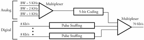

Solution.

Each analog input is sampled by a frequency two times greater than its corresponding bandwidth according to the Nyquist sampling rule. Therefore, we have 5 x 2 + 2 x 2 + 1 x 2 = 16 K samples per second. Once it is encoded, we get a total 16, 000 x 5 = 80 Kb/s on analog lines. The total share of digital lines is then is 170 - 80 = 90 Kb/s. Since each digital line must generate 22.5 Kb/s while the actual rate of 8 Kb/s exists, each digital line must add a difference of 14.5 Kb/s pulse stuffing in order to balance the ultimate bit rate of multiplexer bit rate.

Consider a multiplexer with n available channels. If the number of requesting input sources, m , is greater than n channels, the multiplexer typically reacts by blocking where unassigned sources are not transmitted and therefore remain inactive. Let t _a and t _d be the two mean times during which a given input becomes active and idle, respectively. Assume that the transmission line has n channels available the transmission line but that multiplexer m has inputs, where m>n .

If more than n inputs are active, we can choose only n out of m active sources and permanently block others. If one of the n chosen channels goes to idle, we can give service to one of the other requests . Typically, blocking is used when channels must be held for long time periods. The traditional telephone system is one example; channels are assigned at the start of a call, and other callers are blocked if no channel is available. Assuming that values of t _a and t _d are random and are exponentially distributed, the probability that a source is active, , can be obtained by

Equation 3.1

Let p _j be the probability that j out of m inputs are active; for 1 j m ,

Equation 3.2

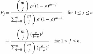
Thus, the probability that j out of n channels on the transmission line are in use, P _j , can be expressed by normalizing p _j over n inputs as or

Equation 3.3

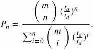
The reason behind the normalization is that can never be equal to 1, since n m ;according to the rule of total probability, we can say only . The blocking probability of such multiplexers, P _n , can be calculated by simply letting j be n in Equation (3.3), denoting that all n channels are occupied. If we also substitute = t _a /( t _d + t _a ), the blocking probability can be obtained when j = n :

Equation 3.4

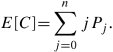
The preceding discussion can be concluded by using basic probability theory to find the average number of busy channels or the expected number of busy channels as

Equation 3.5

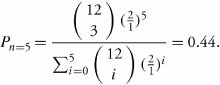
Example.	A 12-input TDM becomes an average of 2 µ s active and 1 µ s inactive on each input line. Frames can contain only five channels. Find the probability that a source is active, , and probability that three channels are in use.
Solution.	We know that m = 12 and n = 5; since t a = 2 µ s, and t d = 1 µ s: and the probability that all five channels are in use is

Statistical TDM

In statistical TDM, a frame's time slots are dynamically allocated, based on demand. This method removes all the empty slots on a frame and makes the multiplexer operate more efficiently. Meanwhile, the trade-off of such a technique is the requirement that additional overhead be attached to each outgoing channel. This additional data is needed because each channel must carry information about which line it belonged to. As a result, in the statistical multiplexer, the frame length is variable not only because of different channel sizes but also because of the possible absence of some channels.

Consider a multiplexer with n available channels. If the number of requesting input sources, m , is greater than n channels, the multiplexer typically reacts by clipping , whereby unassigned sources are partially transmitted, or clipped. Designing multiplexers with m>n stems from the fact that all m sources may not be practically active simultaneously . In some multiplexing systems, clipping is exploited especially for applications in which sources do not transmit continuously, and the best usage of the multiplex output line is targeted . By assigning active sources to channels dynamically, the multiplex output can achieve more efficient channel usage. For example, some satellite or microwave systems detect information energy and assign a user to a channel only when a user is active.

Consider the same definitions as presented in the blocking case for t _a , t _d , m , n ( m> n ), and . Similarly, assume that values of t _a and t _d are random and are exponentially distributed. Assume also that the outgoing transmission line has n channels available but the multiplexer has m inputs, where m>n . If more than n inputs are active, we can dynamically choose n out of m active sources and temporarily block other sources. With temporary blocking, the source is forced to lose, or clip, data for a short period of time, but the source may return to a scanning scenario if a channel becomes free. This method maximizes the use of the common transmission line and offers a method of using the multiplexer bandwidth in silence mode. Note that the amount of data lost from each source depends on t _a , t _d , m , and n . Similar to the blocking case, can be defined by = t _a /( t _d + t _a ), and the probability that exactly k out of m sources are active is

Equation 3.6

Therefore, P _C , the clipping probability, or the probability that an idle source finds at least n sources busy at the time it becomes active, can be obtained by considering all m sources beyond n active sources minus 1 (the examining source):

Equation 3.7

Clearly, the average number of used channels is . The average number of busy channels can then be derived by

Equation 3.8

Example.	For a multiplexer with ten inputs, six channels, and = 0.67, find the clipping probability.
Solution.	Since m = 10, n = 6, P c 0.65.