Section 17.9. Exercises

17.9. Exercises

1.	A sinusoidal signal g(t) with period 10 ms is to be sampled by a sampler s(t) with period T s = 1 ms and pulse width = 0.5 ms. The maximum voltages for both signals are 1 volt. Let the sampled signal be g s (t) ; compute and sketch g(t) , s(t) , g s (t) , G(f) , S(f) , and G s (f) (the range of nT s in s(t) is [-2 T s , +2 T s ]).
2.	Consider a pulse signal g(t) being 1 volt in intervals: ... [-4 and -2], [-1 and +1], [+2 and +4] ... ms. This signal is to be sampled by an impulse sampler s(t) being generated at ..., -3, 0, +3, ... ms, and a convolving pulse c(t) of = 1 volt between -1 and +1 ms. Compute and sketch all the processes from analog signal g(t) to sampled version g s (t) in both time and frequency domains.
3.	Assume that a normal-distributed source with zero mean and variance of 2 is to be transmitted via a channel that can provide a transmission capacity of 4 bits/each source output. What is the minimum mean-squared error achievable? What is the required transmission capacity per source output if the maximum tolerable distortion is 0.05?
4.	Let X(t) denote a normal (Gaussian) source with ƒ 2 = 10, for which a 12-level optimal uniform quantizer is to be designed. Find optimal quantization intervals (”). Find optimal quantization boundaries ( a i ). Find optimal quantization levels . Find the optimal total resulting distortion. Compare the optimal total resulting distortion with the result obtained from the rate-distortion bound that achieves the same amount of distortion.
5.	Consider the same information source discussed in exercise 4. This time, apply a 12-level optimal nonuniform quantizer. Find optimal quantization boundaries ( a i ). Find optimal quantization intervals (”). Find optimal quantization levels . Find the optimal total resulting distortion.
6.	To encode two random signals X and Y that are uniformly distributed on the region between two squares, let the marginal PDF of random variables be 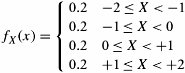and 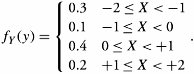Assume that each of the random variables X and Y is quantized using four-level uniform quantizers. Calculate the joint probability P XY (x , y ). Find quantization levels x 1 through x 4 if ” = 1. Without using the optimal quantization table, find the resulting total distortion. Find the resulting number of bits per ( X , Y ) pair.
7.	The sampling rate of a certain CD player is 80,000, and samples are quantized using a 16 bit/sample quantizer. Determine the resulting number of bits for a piece of music with a duration of 60 minutes.
8.	The PDF of a source is defined by f X (x) = 2( x ). This source is quantized using an eight-level uniform quantizer described as follows : 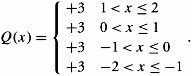Find the PDF of the random variable representing the quantization error X - Q(X) .
9.	Using logic gates, design a PCM encoder using 3-bit gray codes.
10.	To preserve as much information as possible, the JPEG elements of T [ i ][ j ]are divided by the elements of an N x N matrix denoted by D [ i ][ j ], in which the values of elements decrease from the upper-left portion to the lower-right portion. Consider matrices T [ i ][ j ] and D [ i ][ j ] in Figure 17.12. Find the quantized matrix Q [ i ][ j ]. Obtain a run-length compression on Q [ i ][ j ]. Figure 17.12. Exercise 10 matrices for applying (a) divisor matrix D[i][j] on (b) matrix T[i][j] to produce an efficient quantization of a JPEG image to produce matrix Q[i][j]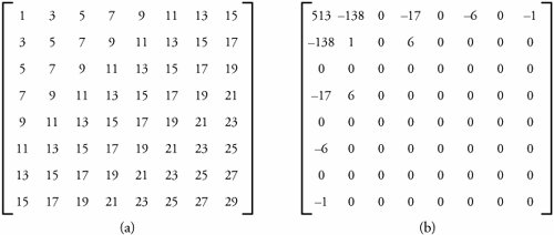
11.	Find the differential entropy of the continuous random variable X with a PDF defined by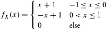
12.	A source has an alphabet { a 1 , a 2 , a 3 , a 4 , a 5 } with corresponding probabilities {0.23, 0.30, 0.07, 0.28, 0.12}. Find the entropy of this source. Compare this entropy with that of a uniformly distributed source with the same alphabet.
13.	We define two random variables X and Y for two random voice signals in a multimedia network, both taking on values in alphabet {1, 2, 3}. The joint probability mass function (JPMF), P X,Y ( x, y ), is given as follows: 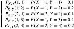Find the two marginal entropies, H(X) and H(Y) Conceptually, what is the meaning of the marginal entropy? Find the joint entropy of the two signals, H(X , Y ). Conceptually, what is the meaning of the joint entropy?
14.	We define two random variables X and Y for two random voice signals in a multimedia network. Find the conditional entropy, H(X Y ), in terms of joint and marginal entropies. Conceptually, what is the meaning of the joint entropy?
15.	Consider the process of a source with a bandwidth W = 50 Hz sampled at the Nyquist rate. The resulting sample outputs take values in the set of alphabet {a , a 1 , a 2 , a 3 , a 4 , a 5 , a 6 } with corresponding probabilities {0.06, 0.09, 0.10, 0.15, 0.05, 0.20, 0.35} and are transmitted in sequences of length 10. Which output conveys the most information? item What is the information content of outputs a 1 and a 5 together? Find the least-probable sequence and its probability, and comment on whether it is a typical sequence. Find the entropy of the source in bits/sample and bits/second. Calculate the number of nontypical sequences.
16.	A source with the output alphabet { a 1 , a 2 , a 3 , a 4 } and corresponding probabilities {0.15, 0.20, 0.30, 0.35} produces sequences of length 100. What is the approximate number of typical sequences in the source output? What is the ratio of typical sequences to nontypical sequences? What is the probability of a typical sequence? What is the number of bits required to represent only typical sequences? What is the most probable sequence, and what is its probability?
17.	For a source with an alphabet { a , a 1 , a 2 , a 3 , a 4 , a 5 , a 6 } and with corresponding probabilities {0.55, 0.10, 0.05, 0.14, 0.06, 0.08, 0.02}: Design a Huffman encoder. Find the code efficiency.
18.	A voice information source can be modeled as a band-limited process with a bandwidth of 4,000 Hz. This process is sampled at the Nyquist rate. In order to provide a guard band to this source, 200 Hz is added to the bandwidth for which a Nyquist rate is not needed. It is observed that the resulting samples take values in the set {-3, -2, -1, 0, 2, 3, 5}, with probabilities {0.05, 0.1, 0.1, 0.15, 0.05, 0.25, 0.3}. What is the entropy of the discrete time source in bits/output? What is the entropy in b/s? Design a Huffman encoder. Find the compression ratio and code efficiency for Part (c).
19.	Design a Lempel-Ziv encoder for the following source sequence: 010100001000111110010101011111010010101010
20.	Design a Lempel-Ziv encoder for the following source sequence: 111110001010101011101111100010101010001111010100001
21.	Computer simulation project . Using a computer program, implement Equation (17.15) to obtain T [ i ][ j ] matrix for a JPEG compression process.