9.4 The M/M/m Queueing Model
The M/M/ m model is a set of mathematical formulas that can predict the performance of queueing systems that meet five very specific criteria. The notation M/M/ m is actually shorthand for the longer notation M/M/ m /  /FCFS, which completely describes all five criteria:
- M /M/ m /
 /FCFS (exponential interarrival time)
 -
The request interarrival time is an exponentially distributed random variable. I shall discuss the meaning of this statement later in this section.
- M/ M / m /
 /FCFS (exponential service time)
 -
The service time is an exponentially distributed random variable.
- M/M/ m /
 /FCFS ( m homogeneous, parallel, independent service channels)
 -
There are m parallel service channels, all of which have identical functional and performance characteristics, and all of which are identically capable of providing service to any arriving service request. For example, in an M/M/1 system, there is a single service channel. In an M/M/32 system, there are 32 parallel service channels.
- M/M/ m /
 /FCFS (no queue length restriction)
 -
There is no restriction on queue length. No request that enters the queue exits the queue until that request receives service.
- M/M/ m /
 / FCFS (first-come, first- served queue discipline)
 -
The queue discipline is first-come, first-served (FCFS). The system honors requests for service in the order in which they were received.
Why "M" Means Exponential You might wonder why queueing theorists use the letter "M" instead of "E" to denote the exponential distribution. It is because "E" denotes another distribution, the Erlang distribution. Faced with the choice of letters other than "E" to denote the exponential distribution, mathematicians chose the letter "M" because the exponential distribution has a unique "Markovian" (or "memoryless") property. Other letters used in this slot for other models include "G" for general, "D" for deterministic, and "H k " for k -stage hyperexponential distributions. |
9.4.1 M/M/m Systems
These five criteria happen to be remarkably fitting descriptions of real phenomena on Oracle systems. M/M/ m queueing systems occur abundantly in the human experience. Examples include:
-
An airport ticket counter where six ticket agents service customers selected from the head of one long, winding queue. This is an M/M/6 system.
-
A four-lane toll road where one toll booth services the cars and trucks selected from the head of a queue that forms in each lane. This is four separate M/M/1 systems, each with an average arrival rate chosen appropriately for each lane.
-
A symmetric multiprocessing (SMP) computer system where twelve CPUs provide service to requests selected from the head of the ready-to-run queue. For reasons of operating system scalability imperfections that I shall discuss later, an appropriate model for this system is M/M/ m , with m chosen in the range 0 < m < 12.
It is clear that all of these examples meet the m ,  , and FCFS criteria of the M/M/ m /
  /FCFS model. But it is less clear without further analysis whether the examples meet the M/M criteria. In the next section, we shall explore what it means to say that a random variable is exponentially distributed.
9.4.2 Non-M/M/m Systems
Even before learning about the M/M criteria, it is easy to see that not all queueing systems are M/M/ m . For example, the following applications are not M/M/ m systems:
-
An airport ticket counter where five ticket agents service airline passengers, but first-class and business class passengers are permitted to cut into the front of the queue. This system violates the FCFS criterion required for the system to be considered M/M/ m .
-
An array of six independent computer disks where each disk services I/O requests from the head of its dedicated queue. This system violates the M/M/6 assumption that all the participating parallel service channels are identically capable of providing service to any arriving service request. For example, a request to read disk D can be fulfilled only by disk D , regardless of what other disks happen to be idle. It is possible to model this system with six independent M/M/1 systems.
-
Oracle latch acquisition. Oracle latches are not allocated to requests in the order the requests are made [Millsap (2001c)]. Therefore Oracle's latch acquisition system violates the FCFS assumption of M/M/ m .
Many systems that fit the .../ m /  /FCFS criteria of queueing systems fail to meet the M/M criteria because their arrival and service processes don't fit the exponential distribution. In the next sections, I shall reveal how to test your operational data for fit to the exponential distribution.
9.4.3 Exponential Distribution
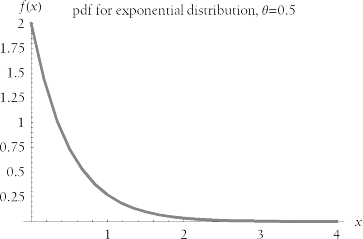
Previously I pointed out that in the early 1900s, Agner Erlang observed that the arrival rate in a telephone system "is Poisson distributed." The phrase "is such-and-such distributed" means only that the probability density function (pdf) of the random variable in question fits a particular mathematical formin this case, the Poisson form. Once we know the pdf of a random variable, we can compute the probability that this random variable will take on any specific value in which we might be interested. To say that a random variable is exponentially distributed with mean q > 0 (the Greek letter theta) is to say that the variable's pdf is of the form:

Figure 9-10 shows the pdf for an exponentially distributed random variable.
Figure 9-10. The pdf for an exponentially distributed random variable with mean q = 0.5
It so happens that many real-life systems have exponentially distributed interarrival times and service times, but we cannot reliably model a system with M/M/ m until we test the system's arrival and service processes. This book provides everything you need to test whether your system's operational characteristics suit the M/M/ m model.
9.4.3.1 Poisson-exponential relationship
Agner Erlang observed that the arrival rate of phone calls in a telephone system obeys a Poisson distribution. Earlier in this section, I commented that many arrival processes in computer systems, including Oracle systems, are Poisson distributed as well. Why, then, would I have chosen to show you the M/M/ m queueing model, which works only if interarrival times and service times are exponentially distributed? Why did I not choose a model in which arrival and service processes were Poisson distributed?
The answer is that, actually, I did choose a model in which arrivals and services were Poisson. The exponential and Poisson distributions bear a reciprocal relationship [Gross and Harris (1998) 16-22]:
-
For a system to suit the criterion defined by the first "M" in "M/M/ m ," its request interarrival times must be exponentially distributed. Remember, however, that the average interarrival time t is the reciprocal of the average arrival rate ( t = 1/ l ). As it happens, an arrival rate with a mean of l is Poisson if and only if the corresponding interarrival time is exponential with mean q = t = 1/ l .
-
For a system to suit the criterion defined by the second "M" in "M/M/ m ," its service times must be exponentially distributed. Of course, the average service time S is the reciprocal of the average service rate ( S = 1/ m ). A service rate with a mean of m is Poisson if and only if the corresponding service time is exponential with mean q = S = 1/ m .
This is why authors sometimes refer to the M/M/ m model as the model for Poisson input and Poisson service.
9.4.3.2 Testing for fit to exponential distribution
The two "M"s of the M/M/ m queueing model notation specify that we can use the model only if the interarrival time and service time are exponentially distributed. That is, we can use M/M/ m to model that system's performance only if the histogram for a system's interarrival times and the histogram for its service rates both resemble the exponential distribution pdf curve shown in Figure 9-10. Figure 9-11 shows some examples.
Figure 9-11. Examples of random data with varying goodness of fit to an exponential distribution with mean q = 0.5
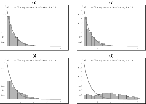
The trick is, how can we tell whether a set of interarrival times or service rates sufficiently "resembles" Figure 9-10? Statisticians use the chi-square goodness-of-fit test to determine whether a list of numbers is sufficiently likely to belong to a specified distribution. The Perl program in Example 9-4 tests whether the numbers stored in a file are likely to be members of an exponential distribution. It produces the verdict "Accept," "Almost suspect," "Suspect," or "Reject" using the procedure recommended in [Knuth (1981) 43-44]. If you have too few data points to perform the chi-square test, the program will tell you. If your operationally measured interarrival times and service times receive a verdict of "Accept" or "Almost suspect," then you can be reasonably certain that the M/M/ m model will produce reliable results.
M/M/ m will make reliable predictions only if interarrival times and service times are both exponentially distributed random variables . Other queueing models produce accurate forecasts for systems with interarrival and service times that are not exponential. I focus here on the M/M/ m model because it is so often well-suited for Oracle performance analysis projects. On Oracle performance projects, it is normally possible to define useful subsets of system workload that meet the M/M criteria. For example:
-
Executions of batch jobs are easy to test for exponentially distributed interarrival times and service times. A good batch queue manager records job request times, job start times, and job completion times for later analysis. A job's interarrival time is simply the difference between the job's request time and the previous job's request time. A job's service time is merely the difference between the job's completion time and the job's start time. By collecting 50 or more interarrival times and 50 or more service times, you can determine whether a given subset of your batch jobs obeys the M/M/ m model's M/M criteria.
The important task here is to use M/M/ m only for a properly behaved subset of your batch data. For example, the interarrival times of your batch jobs over a 24- hour period are likely not to be exponentially distributed: your nighttime interarrival times will likely be much larger than your daytime figures. Likewise, the service times for all of your batch jobs are likely not to be exponentially distributed. However, the service times for all your jobs that execute in less than one minute likely will be approximately exponentially distributed.
-
The Oracle logical I/O (LIO) is a useful unit of measure for service requests. It is not possible to measure LIO interarrival times or service times directly in Oracle, but intuition and a track record of successes using M/M/ m to model LIO performance indicate that LIO interarrival times and service times are indeed exponentially distributed. As long as the execution of each business function can be expressed in terms of an LIO count, you can translate the queueing model's output into terms of business function response time and throughput. Forcing yourself to think of application functions in terms of LIO count is a Very Good Thing.
9.4.3.3 A program to test for exponential distribution
All good queueing theory books inform their readers of the requirement that before you can use the M/M/ m model, you must ensure that the system you're modeling has exponential interarrival times and exponential service times. The problem is that most of these books give you no practical means by which to ensure this. The Perl program shown in Example 9-4 performs the task for you. The idea for the program was inspired by [Allen (1994) 224-225]. Implementation was guided principally by [Knuth (1981) 38-45], with supplemental assistance from Mathematica , [Olkin et al. (1994)], [CRC (1991)], and http://www.cpan.org.
To use this program, download the source code to a system on which Perl is installed. On a Unix (Linux, HP-UX, Solaris, AIX, etc.) system, you'll probably want to name the file mdist . On Microsoft Windows, you'll probably want to call it mdist.pl . On Unix, you may have to edit the top line of the code to refer properly to your Perl executable (e.g., maybe your Perl executable is called /usr/local/bin/perl ). Then type perldoc mdist (or perldoc mdist.pl ) to your command prompt to view the manual page for the program.
Example 9-4. This Perl program tests the likelihood that a random variable is exponentially distributed
#!/usr/bin/perl # $Header: /home/cvs/cvm-book1/mdist/mdist.pl,v 1.7 2002/09/05 23:03:57 cvm # Cary Millsap (cary.millsap@hotsos.com) # Copyright (c) 2002 by Hotsos Enterprises, Ltd. All rights reserved. use strict; use warnings; use Getopt::Long; use Statistics::Distributions qw(chisqrdistr chisqrprob); my $VERSION = do { my @r=(q$Revision: 1.12 $=~/\d+/g); sprintf "%d."."%02d"x$#r,@r }; my $DATE = do { my @d=(q$Date: 2003/11/07 23:13:06 $=~/\d{4}\D\d{2}\D\d{2}/g); sprintf $d[0] }; my $PROGRAM = "Test for Fit to Exponential Distribution"; my %OPT; sub x2($$) { my ($mu, $p) = @_; # The p that &Statistics::Distributions::chisqrdistr expects is the # complement of what we find in [Knuth (1981) 41], Mathematica, or # [CRC (1991) 515]. return chisqrdistr($mu, 1-$p); } sub CDFx2($$) { my ($n, $x2) = @_; # The p that &Statistics::Distributions::chisqrprob returns is the # complement of what we find in [Knuth (1981) 41], Mathematica, or # [CRC (1991) 515]. return 1 - chisqrprob($n, $x2); } sub mdist(%) { my %arg = ( list => [ ], # list of values to test mean => undef, # expected mean of distribution quantiles => undef, # number of quantiles for test @_, # input args override defaults ); # Assign the list. If there aren't at least 50 observations in the # list, then the chi-square test is not valid [Olkin et al. (1994) # 613]. my @list = @{$arg{list}}; die "Not enough data (need at least 50 observations)\n" unless @list >= 50; # Compute number of quantiles and the number of expected observations # for each quantile. If there aren't at least 5 observations expected # in each quantile, then we have too many quantiles [Knuth (1981) 42] # and [Olkin et al. (1994) 613]. my $quantiles = $arg{quantiles} ? $arg{quantiles} : 4; my $m = @list/$quantiles; # we expect quantiles to have identical areas die "Too many quantiles (using $quantiles quantiles reqiures at least ". 5*$quantiles ." observations)\n" unless $m >= 5; # Assign the mean and chi-square degrees of freedom. If no mean was # passed in, then estimate it. But if we estimate the mean, then we # lose an additional chi-square degree of freedom. my $mean = $arg{mean}; my $n_loss = 1; # lose one degree of freedom for guessing quantiles if (!defined $mean) { my $s = 0; $s += $_ for @list; # sum the observed values $mean = $s/@list; # compute the sample mean $n_loss++; # lose additional d.o.f. for estimating the mean } my $n = $quantiles - $n_loss; # chi-square degrees of freedom die "Not enough quantiles for $n_loss lost degrees of freedom (need at least ". ($n_ loss+1) ." quantiles)\n" unless $n >= 1; # Dump values computed thus far. if ($OPT{debug}>=1) { print "list = (", join(", ", @list), ")\n"; printf "quantiles = %d\n", $quantiles; printf "mean = %s\n", $mean; } # Compute interior quantile boundaries. N.B.: The definition of # quantile boundaries is what makes this test for exponential # distribution different from a test for some other distribution. If # the input list is exponentially distributed, then we expect for # there to be $m observations in each quantile, with quantile # boundaries defined at -$mean*log(1-$i/$quantiles) for each # i=1..$quantiles-1. my @q; # list of interior quantile boundaries for (my $i=1; $i<=$quantiles-1; $i++) { $q[$i] = -$mean*log(1-$i/$quantiles); } # Compute frequency of observed values [Knuth (1981) 40]. Setting # $Y[0]=undef makes array content begin at $Y[1], which simplifies # array indexing throughout. my @Y = (undef, (0) x $quantiles); for my $e (@list) { print "e=$e\n" if $OPT{debug}>=3; for (my $i=1; $i<=$quantiles; $i++) { print " i=$i (before): q[$i]=$q[$i]\n" if $OPT{debug}>=3; if ($i = =$quantiles) { $Y[-1]++; print " Y[-1]->$Y[-1]\n" if $OPT{debug}> =3; last } if ($e <= $q[$i]) { $Y[$i]++; print " Y[$i]->$Y[$i]\n" if $OPT{debug}> =3; last } } } # Populate list containing frequency of expected values per quantile # [Knuth (1981) 40]. Using a data structure for this is unnecessarily # complicated for this test, but it might make the program easier to # adapt to tests for other distributions in other applications. (We # could have simply used $m anyplace we mention $np[$anything].) my @np = (undef, ($m) x $quantiles); # Dump data structure contents if debugging. if ($OPT{debug}>=1) { print "mean = $mean\n"; print "q = (", join(", ", @q[1 .. $quantiles-1]), ")\n"; print "Y = (", join(", ", @Y[1 .. $quantiles] ), ")\n"; print "np = (", join(", ", @np[1 .. $quantiles] ), ")\n"; } # Compute the chi-square statistic [Knuth (1981) 40]. my $V = 0; $V += ($Y[$_] - $np[$_])**2 / $np[$_] for (1 .. $quantiles); # Compute verdict as a function of where V fits in the appropriate # degrees-of-freedom row of the chi-square statistical table. From # [Knuth (1981) 43-44]. my $verdict; my $p = CDFx2($n, $V); if ($p < 0.01) { $verdict = "Reject" } elsif ($p < 0.05) { $verdict = "Suspect" } elsif ($p < 0.10) { $verdict = "Almost suspect" } elsif ($p <= 0.90) { $verdict = "Accept" } elsif ($p <= 0.95) { $verdict = "Almost suspect" } elsif ($p <= 0.99) { $verdict = "Suspect" } else { $verdict = "Reject" } # Return a hash containing the verdict and key statistics. return (verdict=>$verdict, mean=>$mean, n=>$n, V=>$V, p=>$p); } %OPT = ( # default values mean => undef, quantiles => undef, debug => 0, version => 0, help => 0, ); GetOptions( "mean=f" => $OPT{mean}, "quantiles=i" => $OPT{quantiles}, "debug=i" => $OPT{debug}, "version" => $OPT{version}, "help" => $OPT{help}, ); if ($OPT{version}) { print "$VERSION\n"; exit } if ($OPT{help}) { print "Type 'perldoc #!/usr/bin/perl # $Header: /home/cvs/cvm-book1/mdist/mdist.pl,v 1.7 2002/09/05 23:03:57 cvm # Cary Millsap (cary.millsap@hotsos.com) # Copyright (c) 2002 by Hotsos Enterprises, Ltd. All rights reserved. use strict; use warnings; use Getopt::Long; use Statistics::Distributions qw(chisqrdistr chisqrprob); my $VERSION = do { my @r=(q$Revision: 1.12 $=~/\d+/g); sprintf "%d."."%02d"x$#r,@r }; my $DATE = do { my @d=(q$Date: 2003/11/07 23:13:06 $=~/\d{4}\D\d{2}\D\d{2}/g); sprintf $d[0] }; my $PROGRAM = "Test for Fit to Exponential Distribution"; my %OPT; sub x2($$) { my ($mu, $p) = @_; # The p that &Statistics::Distributions::chisqrdistr expects is the # complement of what we find in [Knuth (1981) 41], Mathematica, or # [CRC (1991) 515]. return chisqrdistr($mu, 1-$p); } sub CDFx2($$) { my ($n, $x2) = @_; # The p that &Statistics::Distributions::chisqrprob returns is the # complement of what we find in [Knuth (1981) 41], Mathematica, or # [CRC (1991) 515]. return 1 - chisqrprob($n, $x2); } sub mdist(%) { my %arg = ( list => [ ], # list of values to test mean => undef, # expected mean of distribution quantiles => undef, # number of quantiles for test @_, # input args override defaults ); # Assign the list. If there aren't at least 50 observations in the # list, then the chi-square test is not valid [Olkin et al. (1994) # 613]. my @list = @{$arg{list}}; die "Not enough data (need at least 50 observations)\n" unless @list >= 50; # Compute number of quantiles and the number of expected observations # for each quantile. If there aren't at least 5 observations expected # in each quantile, then we have too many quantiles [Knuth (1981) 42] # and [Olkin et al. (1994) 613]. my $quantiles = $arg{quantiles} ? $arg{quantiles} : 4; my $m = @list/$quantiles; # we expect quantiles to have identical areas die "Too many quantiles (using $quantiles quantiles reqiures at least ". 5*$quantiles ." observations)\n" unless $m >= 5; # Assign the mean and chi-square degrees of freedom. If no mean was # passed in, then estimate it. But if we estimate the mean, then we # lose an additional chi-square degree of freedom. my $mean = $arg{mean}; my $n_loss = 1; # lose one degree of freedom for guessing quantiles if (!defined $mean) { my $s = 0; $s += $_ for @list; # sum the observed values $mean = $s/@list; # compute the sample mean $n_loss++; # lose additional d.o.f. for estimating the mean } my $n = $quantiles - $n_loss; # chi-square degrees of freedom die "Not enough quantiles for $n_loss lost degrees of freedom (need at least ". ($n_ loss+1) ." quantiles)\n" unless $n >= 1; # Dump values computed thus far. if ($OPT{debug}>=1) { print "list = (", join(", ", @list), ")\n"; printf "quantiles = %d\n", $quantiles; printf "mean = %s\n", $mean; } # Compute interior quantile boundaries. N.B.: The definition of # quantile boundaries is what makes this test for exponential # distribution different from a test for some other distribution. If # the input list is exponentially distributed, then we expect for # there to be $m observations in each quantile, with quantile # boundaries defined at -$mean*log(1-$i/$quantiles) for each # i=1..$quantiles-1. my @q; # list of interior quantile boundaries for (my $i=1; $i<=$quantiles-1; $i++) { $q[$i] = -$mean*log(1-$i/$quantiles); } # Compute frequency of observed values [Knuth (1981) 40]. Setting # $Y[0]=undef makes array content begin at $Y[1], which simplifies # array indexing throughout. my @Y = (undef, (0) x $quantiles); for my $e (@list) { print "e=$e\n" if $OPT{debug}>=3; for (my $i=1; $i<=$quantiles; $i++) { print " i=$i (before): q[$i]=$q[$i]\n" if $OPT{debug}>=3; if ($i = =$quantiles) { $Y[-1]++; print " Y[-1]->$Y[-1]\n" if $OPT{debug}> =3; last } if ($e <= $q[$i]) { $Y[$i]++; print " Y[$i]->$Y[$i]\n" if $OPT{debug}> =3; last } } } # Populate list containing frequency of expected values per quantile # [Knuth (1981) 40]. Using a data structure for this is unnecessarily # complicated for this test, but it might make the program easier to # adapt to tests for other distributions in other applications. (We # could have simply used $m anyplace we mention $np[$anything].) my @np = (undef, ($m) x $quantiles); # Dump data structure contents if debugging. if ($OPT{debug}>=1) { print "mean = $mean\n"; print "q = (", join(", ", @q[1 .. $quantiles-1]), ")\n"; print "Y = (", join(", ", @Y[1 .. $quantiles] ), ")\n"; print "np = (", join(", ", @np[1 .. $quantiles] ), ")\n"; } # Compute the chi-square statistic [Knuth (1981) 40]. my $V = 0; $V += ($Y[$_] - $np[$_])**2 / $np[$_] for (1 .. $quantiles); # Compute verdict as a function of where V fits in the appropriate # degrees-of-freedom row of the chi-square statistical table. From # [Knuth (1981) 43-44]. my $verdict; my $p = CDFx2($n, $V); if ($p < 0.01) { $verdict = "Reject" } elsif ($p < 0.05) { $verdict = "Suspect" } elsif ($p < 0.10) { $verdict = "Almost suspect" } elsif ($p <= 0.90) { $verdict = "Accept" } elsif ($p <= 0.95) { $verdict = "Almost suspect" } elsif ($p <= 0.99) { $verdict = "Suspect" } else { $verdict = "Reject" } # Return a hash containing the verdict and key statistics. return (verdict=>$verdict, mean=>$mean, n=>$n, V=>$V, p=>$p); } %OPT = ( # default values mean => undef, quantiles => undef, debug => 0, version => 0, help => 0, ); GetOptions( "mean=f" => \$OPT{mean}, "quantiles=i" => \$OPT{quantiles}, "debug=i" => \$OPT{debug}, "version" => \$OPT{version}, "help" => \$OPT{help}, ); if ($OPT{version}) { print "$VERSION\n"; exit } if ($OPT{help}) { print "Type 'perldoc $0' for help\n"; exit } my $file = shift; $file = "&STDIN" if !defined $file; open FILE, "<$file" or die "can't read '$file' ($!)"; my @list; while (defined (my $line = <FILE>)) { next if $line =~ /^#/; next if $line =~ /^\s*$/; chomp $line; for ($line) { s/[^0-9.]/ /g; s/^\s*//g; s/\s*$//g; } push @list, split(/\s+/, $line); } close FILE; print join(", ", @list), "\n" if $OPT{debug}; my %r = mdist(list=>[@list], mean=>$OPT{mean}, quantiles=>$OPT{quantiles}); print " Hypothesis: Data are exponentially distributed with mean $r{mean}\n"; printf "Test result: n=%d V=%.2f p=%.3f\n", $r{n}, $r{V}, $r{p}; print " Verdict: $r{verdict}\n"; _ _END_ _ =head1 NAME mdist - test data for fit to exponential distribution with specified mean =head1 SYNOPSIS mdist [--mean=I<m>] [--quantiles=I<q>] [I<file>] =head1 DESCRIPTION B<mdist> tests whether a random variable appears to be exponentially distributed with mean I<m>. This information is useful in determining, for example, whether a given list of operationally collected interarrival times or service times is suitable input for the M/M/m queueing theory model. B<mdist> reads I<file> for a list of observed values. If no input file is specified, then B<mdist> takes its input from STDIN. The input must contain at least 50 observations. The program prints the test hypothesis, the test results, and a verdict: $ perl mdist.pl 001.d Hypothesis: Data are exponentially distributed with mean 0.000959673232 Test result: n=2 V=0.72 p=0.302 Verdict: Accept The test result statistics [Knuth (1981) 39-45] include: =over 4 =item I<n> Degrees of freedom from the chi-square test. =item I<V> The "chi-square" statistic. =item I<p> The probability at which I<V> is expected to occur in a chi-square distribution with degrees of freedom equal to I<n>. =back B<mdist> uses a I<q>-quantile chi-square test for exponential distribution, adapted from [Allen (1994) 224-225] and [Knuth (1981) 39-40]. Allen provides the strategy for divvying the data into quantiles and testing whether the frequency in each quantile matches our expectation of the exponential distribution. Knuth provides the general chi-square testing strategy that produces a verdict of "Accept", "Almost suspect", "Suspect", or "Reject". =head2 Options =over 4 =item B<--mean=>I<m> The hypothesized expected value of the random variable (i.e., the hypothesized mean of the exponential distribution). If no I<m> is specified, then B<mdist> will use the sample mean of the input and adjust the chi-square degrees of freedom parameter appropriately. =item B<--quantiles=>I<q> The number of quantiles to use in the chi-square test for goodness-of-fit. The number of quantiles must equal at least 2 if a mean is specified, and 3 if the mean will be estimated. The number of quantiles must be small enough that the number of observations divided by I<q> must be at least 5. The default is I<q>=4. =back =head1 AUTHOR Cary Millsap (cary.millsap@hotsos.com) =head1 BUGS Instead of estimating the distribution mean by computing the sample mean, we should probalby use the minimum chi-squared estimation technique described in [Olkin et al. (1994) 617-623]. =head1 SEE ALSO Allen, A. O. 1994. Computer Performance Analysis with Mathematica. Boston MA: AP Professional CRC 1991. Standard Mathematical Tables and Formulae, 29ed. Boca Raton FL: CRC Press Knuth, D. E. 1981. The Art of Computer Programming, Vol 2: Seminumerical Algorithms. Reading MA: Addison Wesley Olkin, I.; Gleser, L. J.; Derman, C. 1994. Probability Models and Applications, 2ed. New York NY: Macmillan Wolfram, S. 1999. Mathematica. Champaign IL: Wolfram =head1 COPYRIGHT Copyright (c) 2002 by Hotsos Enterprises, Ltd. All rights reserved. ' for help\n"; exit } my $file = shift; $file = "&STDIN" if !defined $file; open FILE, "<$file" or die "can't read '$file' ($!)"; my @list; while (defined (my $line = <FILE>)) { next if $line =~ /^#/; next if $line =~ /^\s*$/; chomp $line; for ($line) { s/[^0-9.]/ /g; s/^\s*//g; s/\s*$//g; } push @list, split(/\s+/, $line); } close FILE; print join(", ", @list), "\n" if $OPT{debug}; my %r = mdist(list=>[@list], mean=>$OPT{mean}, quantiles=>$OPT{quantiles}); print " Hypothesis: Data are exponentially distributed with mean $r{mean}\n"; printf "Test result: n=%d V=%.2f p=%.3f\n", $r{n}, $r{V}, $r{p}; print " Verdict: $r{verdict}\n"; _ _END_ _ =head1 NAME mdist - test data for fit to exponential distribution with specified mean =head1 SYNOPSIS mdist [--mean=I<m>] [--quantiles=I<q>] [I<file>] =head1 DESCRIPTION B<mdist> tests whether a random variable appears to be exponentially distributed with mean I<m>. This information is useful in determining, for example, whether a given list of operationally collected interarrival times or service times is suitable input for the M/M/m queueing theory model. B<mdist> reads I<file> for a list of observed values. If no input file is specified, then B<mdist> takes its input from STDIN. The input must contain at least 50 observations. The program prints the test hypothesis, the test results, and a verdict: $ perl mdist.pl 001.d Hypothesis: Data are exponentially distributed with mean 0.000959673232 Test result: n=2 V=0.72 p=0.302 Verdict: Accept The test result statistics [Knuth (1981) 39-45] include: =over 4 =item I<n> Degrees of freedom from the chi-square test. =item I<V> The "chi-square" statistic. =item I<p> The probability at which I<V> is expected to occur in a chi-square distribution with degrees of freedom equal to I<n>. =back B<mdist> uses a I<q>-quantile chi-square test for exponential distribution, adapted from [Allen (1994) 224-225] and [Knuth (1981) 39-40]. Allen provides the strategy for divvying the data into quantiles and testing whether the frequency in each quantile matches our expectation of the exponential distribution. Knuth provides the general chi-square testing strategy that produces a verdict of "Accept", "Almost suspect", "Suspect", or "Reject". =head2 Options =over 4 =item B<--mean=>I<m> The hypothesized expected value of the random variable (i.e., the hypothesized mean of the exponential distribution). If no I<m> is specified, then B<mdist> will use the sample mean of the input and adjust the chi-square degrees of freedom parameter appropriately. =item B<--quantiles=>I<q> The number of quantiles to use in the chi-square test for goodness-of-fit. The number of quantiles must equal at least 2 if a mean is specified, and 3 if the mean will be estimated. The number of quantiles must be small enough that the number of observations divided by I<q> must be at least 5. The default is I<q>=4. =back =head1 AUTHOR Cary Millsap (cary.millsap@hotsos.com) =head1 BUGS Instead of estimating the distribution mean by computing the sample mean, we should probalby use the minimum chi-squared estimation technique described in [Olkin et al. (1994) 617-623]. =head1 SEE ALSO Allen, A. O. 1994. Computer Performance Analysis with Mathematica. Boston MA: AP Professional CRC 1991. Standard Mathematical Tables and Formulae, 29ed. Boca Raton FL: CRC Press Knuth, D. E. 1981. The Art of Computer Programming, Vol 2: Seminumerical Algorithms. Reading MA: Addison Wesley Olkin, I.; Gleser, L. J.; Derman, C. 1994. Probability Models and Applications, 2ed. New York NY: Macmillan Wolfram, S. 1999. Mathematica. Champaign IL: Wolfram =head1 COPYRIGHT Copyright (c) 2002 by Hotsos Enterprises, Ltd. All rights reserved. 9.4.4 Behavior of M/M/m Systems
The beauty of M/M/ m is that using the model makes it possible to experiment with parameters that would be very expensive to manipulate in the real world. In this section, we'll examine a few interesting behaviors of M/M/ m . These model behaviors will help explain how to avoid some of the undesirable performance behaviors that plague real multi-channel queueing systems. The result will be a clearer understanding of the Oracle system you're probably thinking about right now.
9.4.4.1 Multi-channel scalability
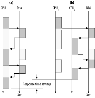
Of course, two CPUs are better than one. But why? And under what circumstances? An easy way to conceptualize the answer is to use a sequence diagram. Figure 9-12 reveals the answer. On the system shown in case a , the first disk I/O call cannot return immediately to the single CPU because that CPU is occupied doing other work. Thus, the CPU request queues, which of course increases response time. The system shown in case b has two CPUs. When the disk I/O call returns, it finds CPU 1 busy, but CPU 2 is ready and able to service the request, which results in the elimination of a queueing delay, which improves response time for the business function. Note the interesting effect of creating a new bottleneck on the disk in case b .
Figure 9-12. More service channels (in this drawing, CPUs) improve response times on busy systems by reducing queueing delays
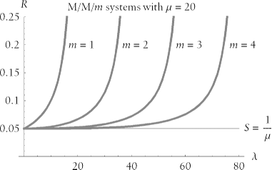
This phenomenon of reduced queueing in systems with larger m manifests itself clearly in the output of M/M/ m . Figure 9-13 shows the performance effect of increasing the number of parallel service channels. Although the service time ( S ) remains constant across all the systems represented by the figure, response times ( R ) are smaller at higher arrival rates ( l ) on systems with more service channels ( m ), because there is less queueing delay ( W = R - S ).
Figure 9-13. Increasing the number of parallel service channels provides greater capacity to arrivals requesting service, which reduces response time at higher arrival rates
So, which is better, a system with a single very fast CPU? Or a system with m > 1 slower CPUs? Most consultants have the correct answer programmed into their RNA: "It depends." But with M/M/ m you have the tools to answer the very good question, "On what ?"
Figure 9-14 shows very clearly that the "it depends" depends only upon one variable: the arrival rate. For low arrival rates, an m = 1 system with the fast CPU will provide superior performance. For high arrival rates, the m > 1 system will be faster. You can estimate the break-even point l eq by inspection if you plot the response time curves in a tool like you can find at http://www.hotsos.com. If you want a more detailed answer, you could find the l value for which the two systems' response times are equal by using the interval bisection method shown earlier in the LambdaMax function of Example 9-2. Or you can compute l eq symbolically with a tool like Mathematica .
Figure 9-14. A computer with a single fast CPU produces better response times for low arrival rates, but a computer with four slower CPUs produces better response times for high arrival rates
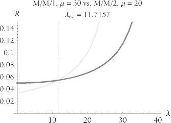
People who have tried both types of system notice the behavior depicted in Figure 9-14 in very practical terms:
-
A long nightly batch job runs faster on the system with the single fast CPU. This result often surprises people who "upgrade" from the single-CPU system to the multi-CPU system. But when a single-threaded job runs solo on a system, the arrival rate is low. It will run the fastest on a fast CPU. The multi-CPU system doesn't provide reduction in queueing delay on a system with a low arrival rate, because on such a system there is no queueing to begin with.
-
The multi-CPU system provides better response times to online users during their busiest work hours. This result is due to the reduction in queueing that a multi-channel system provides. Multi-CPU systems scale better to high arrival rates (such as those induced by high concurrent user counts) than single-CPU systems.
Naturally, the better system to purchase depends upon an array of both technical and non-technical factors, including price, hardware reliability, dealer service, upgrade flexibility, and compatibility with other systems. But the expected peak arrival rate of workload into your system, which is profoundly influenced by your system's concurrency level, should definitely factor into your decision.
9.4.4.2 The knee
The most interesting part of the performance curve is its "knee." Intuitively, the location of the "knee in the curve" is the utilization value at which the curve appears to starting going up faster than it goes out . Unfortunately , this intuitive definition doesn't work, because the apparent location of the knee changes, depending on how you draw the curve. Figure 9-15 illustrates the problem. The graphs shown here are two different plots of the same response time curve. The only difference between the two plots is the scale of the vertical axis. The visual evidence presented here is overwhelming: clearly "these two systems have different knees." But remember, they are not two systems, they are plots of the same system using different vertical scales .
Figure 9-15. Two views of the exact same graph plotted using two different vertical scales. Intuitively, it appears that the knee in the top curve occurs at r  0.8 and that the knee in the bottom curve occurs to the right of
To visually seek the utilization at which the "greatest bend occurs" is thus an unreliable method for locating the knee. Obviously, a useful definition of a system's "knee" cannot rely upon an arbitrary selection of which drawing unit an artist chooses for a plot of the system's response time curve.
 | One author gets this point terribly wrong in his paper Performance Management: Myths & Facts [Millsap (1999) 8]. The points he was trying to make are indeed relevantthere in fact is a knee in the response time curve, and in fact the knee does move rightward as you add service channels. However, the author's definition of knee (the r value "at which the curve begins to go `up' faster than it goes `out') is unfortunately the intuitive one that is debunked above. And the manner in which he suggested that the knee might be found (calculating the value of r for which  R / R /  knee of the response time curve occurs at the utilization value r * (rho-star) at which the ratio R / r achieves its minimum value. Graphically, the location of the knee is the utilization ( r ) value at which a straight line drawn through the origin touches the response time curve in exactly one point, as shown in Figure 9-16. Many analysts consider the value r * the optimal utilization for an M/M/ m system, because... knee of the response time curve occurs at the utilization value r * (rho-star) at which the ratio R / r achieves its minimum value. Graphically, the location of the knee is the utilization ( r ) value at which a straight line drawn through the origin touches the response time curve in exactly one point, as shown in Figure 9-16. Many analysts consider the value r * the optimal utilization for an M/M/ m system, because... ...it is usually desirable to simultaneously minimize R (to satisfy users) and maximize r (to share resource cost among many users) [Vernon(2001)]. As we have seen, for utilization values to the left of the knee (for r < r *), we waste system capacity. After all, if we're running at low utilization, we can add workload without appreciably degrading response times. For utilization values to the right of the knee (for r > r *), we risk inflicting serious response time degradation upon our users even for tiny fluctuations in workload. Figure 9-16. The knee is the utilization value r * at which R/ r achieves its minimum value. Equivalently, the knee is the r value at which a line through the origin is tangent to the response time curve 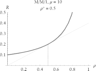 The location of the knee in an M/M/ m system is a function solely of m , the number of parallel service channels. As we've seen, adding parallel service channels will allow a system to run at higher utilization values without appreciable response time degradation. Figure 9-17 shows how the location of the knee moves rightward in the utilization domain as we increase the value of m . Figure 9-17. The knee value moves rightward in the utilization domain ( r ) as the number of parallel service channels (m) increases 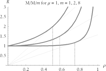 The location of the knee for a given value of m is constant, regardless of service rate. This phenomenon is demonstrated in Figure 9-18. In this figure, changes to the service rate ( m ) motivate changes to response times (note the differing labels on the R axis), but the shape of the performance curve and location of the knee are the same for all M/M/1 systems. Similarly, all M/M/2 curves share a single shape and a single knee value. All M/M/3 curves share a single shape and a single knee value, and so on.  | Two curves f 1 and f 2 can be said to have the same shape if f 1 ( x ) = k f 2 ( x ) at every x for some constant k . That is, two curves have the same shape if they can be made to look identical by scaling one curve's vertical axis by a constant. | | Figure 9-18. The location of the knee is constant for a given m, regardless of the value of m. Under conditions of service rate changes, the vertical position of the curve moves, but neither the curve's shape nor its knee location changes 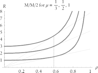 Because all M/M/ m systems with a fixed value of m have an identical knee utilization, it is possible to create a table that lists the location of the knee for interesting values of m . Table 9-3 shows the location of the knee for various M/M/ m systems. Table 9-3. The utilization value r * at which the knee occurs in an M/M/m system depends upon the value of m | m | r * | | m | r * | | 1 | 0.5 | | 32 | 0.86169 | | 2 | 0.57735 | | 40 | 0.875284 | | 3 | 0.628831 | | 48 | 0.885473 | | 4 | 0.665006 | | 56 | 0.893482 | | 5 | 0.692095 | | 64 | 0.899995 | | 6 | 0.713351 | | 80 | 0.910052 | | 7 | 0.730612 | | 96 | 0.917553 | | 8 | 0.744997 | | 112 | 0.923427 | | 16 | 0.810695 | | 128 | 0.928191 | | 24 | 0.842207 | | | | Table 9-4 gives further insight into the performance of M/M/ m systems. It illustrates how average response time degrades relative to utilization on various M/M/ m systems. For example, if the average response time on an unloaded M/M/1 system is R = S seconds, then the average response time will degrade to R = 2 S seconds (twice the unloaded response time) when utilization reaches 50%. Response time will degrade to four times the unloaded response time when utilization reaches 75%, and to ten times the unloaded response time when utilization reaches 90%. On an M/M/8 system, response time will degrade to R = 4 S seconds only when system utilization reaches 96.3169%. These figures match the intuition acquired by studying the effects of adding service channels upon response time scalability. Table 9-4. The utilization on M/M/m systems at which response time becomes k times worse than the service time (that is, at which R = kS) | k | m | | | 1 | 2 | 4 | 8 | 16 | | 1 | 0. | 0. | 0. | 0. | 0. | | 2 | 0.5 | 0.707107 | 0.834855 | 0.909166 | 0.950986 | | 3 | 0.666667 | 0.816497 | 0.901222 | 0.947673 | 0.97263 | | 4 | 0.75 | 0.866025 | 0.929336 | 0.963169 | 0.980984 | | 5 | 0.8 | 0.894427 | 0.944954 | 0.971569 | 0.985426 | | 6 | 0.833333 | 0.912871 | 0.954907 | 0.976844 | 0.988184 | | 7 | 0.857143 | 0.92582 | 0.961807 | 0.980467 | 0.990064 | | 8 | 0.875 | 0.935414 | 0.966874 | 0.983109 | 0.991427 | | 9 | 0.888889 | 0.942809 | 0.970753 | 0.985121 | 0.992462 | | 10 | 0.9 | 0.948683 | 0.973818 | 0.986704 | 0.993273 | 9.4.4.3 Response time fluctuations Online system users who execute the same task over and over are very sensitive to fluctuations in response time. Given a choice, most users would probably prefer a consistent two-second response time for an online form over response time that averages two seconds per form but does so by providing sub-second response for 75% of executions and seven-second response time for 25% of executions. You have perhaps noticed that on low-load systems, response times are mostly stable, but on very busy systems, response times can fluctuate wildly. The queueing model explains why. Figure 9-19 depicts the very small degradation in response time (from R 1 to R 2 ) of a multi-channel (i.e., m > 1) system as its utilization increases from r 1 to r 2 . Notice how the R 1 and R 2 values are so close together that their labels overlap. However, to right of the knee, even a very tiny change in utilization from r 3 to r 4 produces a profound degradation in response time (from R 3 to R 4 ). Figure 9-19. Left of the knee, response time is insensitive even to large fluctuations in utilization, but right of the knee, even tiny fluctuations in utilization create huge response time variances 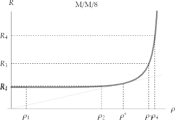 As we learned in the previous section, multi-channel systems can provide stable response times for higher arrival rates than single-channel systems can handle. The excellent scalability shown in Figure 9-19 is another illustration of this phenomenon. However, the capacity of even the largest multi-channel system is finite, and when the arrival rate begins to encroach upon that finite limit of capacity, performance degrades quickly. By contrast, performance of single-channel systems degrades more smoothly, as shown in Figure 9-20. In this picture, response time clearly degrades faster to the right of the knee. However, in systems with few parallel service channels (i.e., with small m ), the degradation is distributed more uniformly throughout the entire range of utilization values than it is for systems with many parallel service channels (i.e., with large m ). Figure 9-20. Response time degrades more uniformly throughout the domain of utilization values on single-channel (and small-m) systems 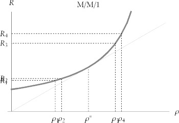 A single-channel queueing system is less scalable than a similarly loaded queueing system with multiple service channels. That is, its knee is nearer to the low end of the utilization domain. But every system has a knee. Especially on highly scalable multi-channel systems, once you drive workload past the knee, the system's users are in for a wild ride of fluctuating response times. Bad CPU Utilization Targets I am reluctant to express a " good CPU utilization target" because CPU utilization is a side-effect of the metric to which you really should be targeting: response time. However, avoiding some bad utilization values can help keep you out of system performance trouble. -
On batch-only application systems, CPU utilization of less than 100% is bad if there's work waiting in the job queue. The goal of a batch-only system user is maximized throughput . If there's work waiting, then every second of CPU capacity left idle is a second of CPU capacity gone wasted that can never be reclaimed. But be careful: pegging CPU utilization at 100% over long periods often causes OS scheduler thrashing, which can reduce throughput. -
On interactive-only application systems, CPU utilization that stays to the right of the knee over long periods is bad. The goal of an interactive-only system user is minimized response time . When CPU utilization exceeds the knee in the response time curve, response time fluctuations become unbearable. By leaving idle capacity on the system, the system manager effectively purchases better response time stability. -
On systems with a mixture of batch and interactive workload, your job is much more difficult, because your users' performance goals are contradictory. On mixed-workload systems, it is important for you to prioritize your workloads. If interactive response time is more important, then you'll want to ensure that you don't drive CPU utilization too far to the right of the knee. If batch throughput is more important, then you'll not want to waste as much CPU capacity to provide response time stability to your less important users. I discuss a method for determining the optimal mixture of batch and interactive workload in [Millsap (2000b)]. | 9.4.4.4 Parameter sensitivity Spreadsheet-based systems like Microsoft Excel allow you to test what-if situations at a pace that Agner Erlang would have envied. Such what-if tests can save countless iterations through emotional roller coaster rides with end users. For example, on very many occasions in my career, customers have engaged my services to determine why a performance improvement project has failed. Application of the M/M/ m queueing model in several of these occasions has enabled me to explain quickly and concisely why some hardware upgrade didn't produce the desired overall performance improvement. The queueing model has often led to proofs of assertions in forms like: ...This is why upgrading to 100% faster CPUs did not produce the desired performance improvement. Furthermore, even if you could have quadrupled the number of these faster CPUs, you still would not have achieved the desired performance improvement. The only way to produce the desired performance improvement is either to reduce the number of times you use this function, or to reduce the length of the code path that is executed when you use it. In cases like this, earlier use of the queueing model might have averted the catastrophe that had motivated my presence. Using the M/M/ m queueing model in a spreadsheet teaches you that every input parameter and every output parameter of the model is negotiable. The key to optimizing the performance of a system is to understand how the parameters relate to each other, and to understand the economic impact of the choices you can make about each parameter. Each of the following items describes a negotiable parameter and some of the choices you can make about it: - l
-
The arrival rate l is a negotiable parameter that can provide significant leverage to the performance analyst. Many analysts fail even to consider negotiating workload with end users; they assume that the amount of work that the business needs from the system is fixed. But in many cases, a principal cause of system performance trauma is unnecessary workload. Examples include: -
An application sends scheduled alerts via email to each user every two minutes, but each end user reads alerts only twice a day. Thus, the arrival rate for alerts could be reduced by a factor of 120, from 30 alerts per hour to 0.25 alerts per hour. -
A system with eight CPUs becomes extremely slow for its online users from 2:00 p.m. to 3:00 p.m. A prominent workload element during this time period is a set of 16 reports (batch jobs), each of which consumes about 30 minutes of CPU time. The reports will not be read until 8:00 a.m. the next day. Thus, scheduling the 16 batch jobs to run at midnight instead of online business hours would reduce the arrival rate of CPU service requests by enough to conserve about eight CPU-hours of capacity during the 2:00 p.m. to 3:00 p.m. window. -
Accountants generate 14 aged trial balance reports each day to determine whether debits properly match credits in a set of books. Each 200-page report requires the execution of 72,000,000 Oracle logical read calls (LIOs), which consume about 30 minutes of CPU time. However, unbeknownst to the users, the application provides a web page that can tell them everything they need to know about out-of-balance accounts with fewer than 100 LIOs. Thus, the arrival rate of LIOs for this business requirement can be reduced from about one billion per day to about 1,400. What is the fastest way to do something? Find a way to not do it at all. Many times, you can accomplish this goal with no functional compromise to the business. - r max
-
It is possible that users will agree to compromise on their tolerance for spikes in response time, especially if a small compromise in response time tolerance might save their company a lot of money. However, users will quickly tire of attempts to convince them that they should be more tolerant of poor system performance. Unless it is absolutely necessary to find more breathing room, negotiating r max is one of the last places you should seek relief. - p
-
As with negotiations about r max , users are likely to find negotiations about p , the proportion of response times that must not exceed r max , to be counterproductive and frustrating. - q
-
Although the number q of M/M/ m queueing systems is technically a negotiable parameter, scaling an Oracle application system across more than one database server is, even with Oracle9 i Real Application Clusters (RAC), still a technologically challenging endeavor that is almost certain to cost more than a configuration in which the database runs on only a single host. - m
-
The number m of parallel service channels in a system is negotiable, subject to physical constraints and scalability constraints that are imposed chiefly by the operating system. For example, a given system may require that CPUs be installed in multiples of two, up to 32 CPUs, but a 32-CPU system may be only as powerful as a theoretical system with 24 perfectly scalable CPUs. Benchmarks and discussions with vendor scientists can reveal these types of data. - m
-
The service rate m is a negotiable parameter that provides immense leverage to the performance analyst. Many analysts' first impulse for optimizing a system is to improve (increase) m by providing faster hardware. For example, upgrading to 20% faster CPUs should produce a CPU service rate increase on the order of 20%, which can be enormously beneficial for CPU constrained applications. However, what many analysts overlook is the even more important idea that service rate can be improved by reducing the amount of code path required to perform a given business function. In Oracle application systems, performance analysts can often achieve spectacular code path reduction by engaging in the task of SQL optimization . SQL optimization consists of manipulating some combination of schema definitions, database or instance statistics, configuration parameters, query optimizer behavior, or application source code to produce equivalent output with fewer instructions on the database server. Code path reduction has several advantages over capacity upgrades, including: - Cost
-
Capacity upgrades frequently motivate not only the procurement cost of the upgraded components , but also increased maintenance costs and software license fees. For example, some software licenses cost more for systems with n + 1 CPUs than they do for systems with n CPUs. Code path reduction for inefficient SQL statements generally requires no more than a few hours of labor per SQL statement. - Impact
-
Code path reduction often provides far greater leverage to the performance analyst than capacity upgrades. For example, it may be possible to double CPU speeds only once every two years . It is frequently possible to reduce code path length by factors of 105 or more with just a few hours of labor. - Risk
-
Code path reduction carries very little risk of unintended negative side effects that sometimes accompany a capacity upgrade. One possible side effect of a capacity upgrade is performance degradation of programs that were bottlenecked on a device other than one to which the upgrade was applied [Millsap (1999)]. Working even briefly with a queueing model reveals why eliminating unnecessary workload creates such spectacular system-wide performance leverage. The two ways to eliminate work are to eliminate business functions that do not legitimately add value to the business, and to eliminate unnecessary code path. These "two" endeavors are really a single waste-elimination task executed at different layers in the technology stack. 9.4.5 Using M/M/m: Worked Example A worked example provides a good setting for exploring how to use the model and interpret its results. I encourage you to step through the problem that follows while using the M/M/ m queueing theory model (a Microsoft Excel workbook) that is available at http://www.hotsos.com. The problem is a conceptually simple one, but its solution requires an understanding of queueing theory. Here is the problem statement: An important SQL statement consumes 0.49 seconds of CPU service time to execute. We anticipate that each of 100 users will execute this statement at a rate of four times per minute during the system's peak load. The Linux server is equipped with boards that allow installation of up to 16 CPUs. How many CPUs will be required on this Linux server if our goal is to provide sub-second CPU response times in at least 95% of users' executions during peak load? Let's go. 9.4.5.1 Suitability for modeling with M/M/m The first thing you need to do is check whether the system under analysis is suitable for modeling with the M/M/ m /  /FCFS (or M/M/ m for short) queueing model: /FCFS (or M/M/ m for short) queueing model: - M /M/m/
 /FCFS (exponential interarrival time) /FCFS (exponential interarrival time) -
If request interarrival times (the duration between arrivals) are operationally measurable, then your first step is to test whether the interarrival times are exponential by using the program shown in Example 9-4. If your interarrival times are not exponential, then consider modeling a smaller time window. For example, in Case I of the restaurant example I described earlier (reproduced here as Table 9-5), interarrival times are clearly not exponential when regarded over the observation period from 11:30 a.m. to 1:30 p.m. However, interarrival times are much more likely to be exponential over the period from 12:00 noon to 12:15 p.m. Table 9-5. Two very different scenarios both lead to an expected interarrival time of t = 30 seconds | | Number of arrivals | | Time interval | Case I | Case II | | 11:30 a.m. to 11:45 a.m. | | 34 | | 11:45 a.m. to 12:00 noon | | 28 | | 12:00 noon to 12:15 p.m. | 240 | 31 | | 12:15 p.m. to 12:30 p.m. | | 37 | | 12:30 p.m. to 12:45 p.m. | | 24 | | 12:45 p.m. to 1:00 p.m. | | 30 | | 1:00 p.m. to 1:15 p.m. | | 32 | | 1:15 p.m. to 1:30 p.m. | | 24 | | Average per 0:15 bucket | 30 | 30 | If request interarrival times are not operationally measurable (for example, because the system has not yet been designed), then you have to use your imagination . It is almost always possible to construct a time window in which you can confidently assume that interarrival times will be exponential (or, equivalently, that the rate of arrivals will be Poisson). Let's assume for this example that the arrivals can be confirmed operationally as being Poisson. - M/ M / m /
 /FCFS (exponential service time) /FCFS (exponential service time) -
Similarly, you must ensue that service times are exponentially distributed, using the program shown in Example 9-4 or by some other means. If your service times are not exponentially distributed, then consider redefining your service unit of measure. For example, if you define your service unit of measure as a report , but your reports range in service duration from 0.2 seconds to 1,392.7 seconds, the report service times are probably not exponential. Change your service unit of measure to a particular type of report whose service times have less fluctuation. Or reduce your unit of measure to a more "sub-atomic" level, by choosing a unit of measure like the Oracle LIO. In this example, let's assume that we have confirmed by using operational measurements upon a test system that the "important SQL statement" produces service times that are exponentially distributed. - M/M/ m /
 /FCFS ( m homogeneous, parallel, independent service channels) /FCFS ( m homogeneous, parallel, independent service channels) -
The problem statement specifies that our service channel of interest is the CPU on a computer running the Linux operating system. Because Linux is a fully symmetric multiprocessing (SMP) operating system, then we know our service channels to be homogenous, parallel, and independent. Some operating system configurations, such as those that use processor affinity, violate the CPU homogeneity constraint. As you shall soon see, we will also have to account for scalability imperfections when we use the model. We will end up using an M/M/ m model to forecast the performance of a system with more than m CPUs. - M/M/ m /
 /FCFS (no queue length restriction) /FCFS (no queue length restriction) -
A Linux CPU run queue has no relevant depth constraints, so we're clear for takeoff on the "  attribute of the M/M/ m definition. attribute of the M/M/ m definition. - M/M/ m /
 / FCFS (first-come, first-served queue discipline) / FCFS (first-come, first-served queue discipline) -
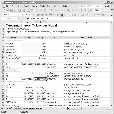
The standard Linux process scheduling policy is approximately first-come, first-served. Even though the scheduling algorithm permits process prioritization and selection from different policies (FCFS and round- robin ), the M/M/ m model has proven suitable for predicting performance of Linux systems. 9.4.5.2 Computing the required number of CPUs The problem statement specifies that our job is to determine the number of CPUs required to meet a particular performance goal. We can set up the problem in the input cells of the Excel M/M/ m workbook as shown in Table 9-6. You will enter the values from the Value column into the yellow cells of the Multiserver Model worksheet of the MMm.xls workbook. Table 9-6. Queueing model input parameters | Name | Valuea | Explanation | | jobunit | stmt | The focal unit of work specified in the problem statement is "an important SQL statement." | | timeunit | sec | Both the response time tolerance and the SQL statement's CPU service time are expressed in seconds . | | queueunit | system | The problem specifies that we are searching for the number of CPUs that we will need to install in a single system. | | serverunit | CPU | The server unit in the problem statement is the CPU. | | l | =100*4/60 | "We anticipate that each of 100 users will execute this statement at a rate of four times per minute during the system's peak load." | | r max | 1 | The goal is to provide response times less than 1.0 second ("...provide sub-second CPU response times"). | | q | 1 | The problem statement specifies that we are to assess a single system. | | m | 1 | The number of CPUs per system is the value that we are seeking. We can enter the value 1 into this cell , because we shall seek shortly for a suitable value. | | m | =1/0.49 | "An important SQL statement consumes 0.49 seconds of CPU service time to execute." Therefore, the service rate is 1/0.49 statements per second. | Once we load these values into the workbook, we see that a configuration with only one CPU ( m = 1) will definitely not handle the required workload (Figure 9-21). Figure 9-21. A one-CPU system will produce sub-second response times in zero percent of cases on a system with l = 6.667 stmt/sec and m = 2.041 stmt/sec. Note that the high arrival rate and comparatively low service rate would drive CPU utilization to 326.7%, a value that is possible only in theory 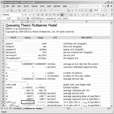 The model predicts that if we equip our system with only one CPU, then keeping up with the 6.67 statements per second coming into the system would require an average CPU utilization of 326.7%. It is of course impossible to run CPU utilization to more than 100%. In reality, such a system would sit at 100% utilization forever. Arrivals would enter the system faster than it can process them, causing the system's queue length to grow continuously and without bound. However, this statistic does give us a clue that we would need to configure our system with at least four CPUs just to provide any chance of the system's keeping up with its workload. The MMm workbook conveniently provides two columns ( value a and value b ) that enable us to see the behavior of two systems side-by-side. If you try the model using m = 4, you'll see the results shown in Figure 9-22. Figure 9-22. Using four perfectly scalable CPUs would cause the system to meet the performance target in 64.9% of cases 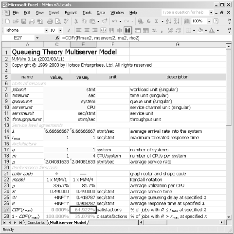 An ideal four-CPU system would produce an average response time of 0.908787 sec/stmt. However, we're still in trouble, because this configuration will provide sub-second response time in only 64.922% of executions of the statement. The original specification required sub-second response time in 95% of executions during peak load. Let's see the theoretical best performance that could happen with the number of CPUs in the machine set to the maximum of m = 16, as shown in Figure 9-23. It turns out that this project is in big, big trouble. Even with the number of CPUs set to m = 16, it is impossible to create user satisfaction with a sub-second response time expectation in more than about 87% executions of the statement. You can try the model yourself: even if we could crank up the configuration to m = 1000, this system still wouldn't be able to provide satisfactory performance in more than about 87% of executions. Figure 9-23. Even with sixteen perfectly scalable CPUs, this system can meet the performance target in only 87% of cases 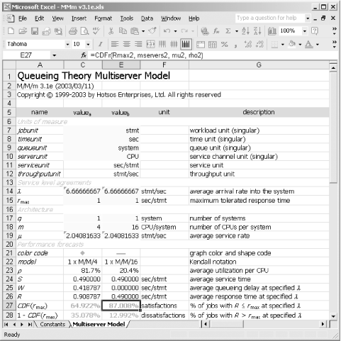 9.4.5.3 What we can learn from an optimistic model Note that the M/M/ m model will allow you to hypothesize the existence of systems that cannot exist in reality. You could, for example, model a perfectly scalable 1,000-CPU Linux system, or even a perfectly scalable 4-CPU Microsoft Windows NT system. No matter how preposterous the input values you enter, the queueing model will faithfully report to you how a perfectly scalable hypothetical system of this configuration would perform. In fact, the model doesn't actually even know whether you are modeling computer systems, grocery stores, or toll booths. It is up to you to decide whether the system you're hypothesizing is feasible to construct. The M/M/ m queueing theory model, used like we have described here, is optimistic because it omits any understanding of real-life barriers to scalability other than the effects of queueing. The upshot of this understanding is significant. If this queueing theory model tells you that something can be done, then it's possible that you still might not be able to do that thing. You can, after all, tell the model that you can cram 1,000 CPUs into a Linux box, and that all this capacity will operate full-strength, no problem. However, if this queueing theory model tells you that something cannot be done, you can take that advice all the way to the bank. If an optimistic model advises you that something is impossible, then it is impossible.  | The M/M/ m model implemented in my Excel workbook is optimistic because it omits any understanding of real-life barrier to scalability other than the effects of queueing. Consequently, for the model to advise you that something can be done does not constitute a proof that your project will succeed. However, for the model to advise you that something cannot be done is sufficient evidence that you cannot do it, as long as your input assumptions are valid. | | Our model has told us that no matter how many CPUs we might add to our hypothetical configuration, we will never be able to meet the performance criterion that 95% of statement executions must finish in sub-second time. This might sound like bad news for the project, but it's immensely better to find out such an unpleasant truth using an inexpensive queueing model than to watch a project fail in spite of vast investments in attempt to make it succeed. 9.4.5.4 Negotiating the negotiable parameters So, confronted with news that our project is doomed, what can we do? One more hidden beauty of queueing theory is that it reveals exactly which system manipulations ( modeled as M/M/ m parameter changes) might make a positive performance impact. I listed the negotiable parameters for you earlier in Section 9.4.4.4. An analysis of those negotiable parameters for this example should include: - Number of systems q , and number of CPUs per system m
-
First, we can investigate a curious output of the model to understand why adding CPUs doesn't seem to increase the response time CDF beyond about 87%. The model shows that even a hundred systems with a hundred CPUs each will not produce satisfactory response times for the statement more than about 87% of the time. The reason is that the service time in an M/M/ m model is a random variable. Although the average service time is a constant, actual service times for a given type of function fluctuate from one function to the next. For example, two identical SQL queries with differing bind values in a where clause predicate might motivate slightly different LIO counts, which will motivate different CPU service times. By increasing the number of CPUs on a system, we reduce only the average queueing delay ( W ) component of response time ( R = S + W ). If the average service time alone is sufficiently near the response time tolerance, then random fluctuations in service times will be enough to cause response time to exceed the specified tolerance for a potentially significant proportion of total executions. There is virtually no benefit to be gained by using more than about six CPUs for this problem's important SQL statement. - Average arrival rate l
-
Does the business really need 100 users each running the important statement four times a minute? It is a legitimate question. In many situations, the best system optimization step to perform first is to realize that the users are asking the machine to do more work than the users could even use. For example, polling a manufacturing process and generating a user alert up to four times a minute is senseless if the user is getting his job done perfectly well by reviewing alerts only once an hour. If the average arrival rate at peak load in our problem could be reduced similarly, from:  statements per second to:  statements per second, it would reduce the workload generated by this statement by a factor of 240. The result would be a significant scalability benefit. The system would require only one CPU to produce satisfactory response times for 87% of the statement's executions. Because the arrival rate l = A / T is a ratio, there are two ways that you can reduce its value. One way is to reduce the numerator A , the number of arrivals into the system, as I've suggested already. Another way is to increase the denominator T , the time period in which the system is required to absorb the specified number of arrivals. Reducing the average arrival rate can enable us to use a less expensive system, but we would still have some work to do. None of the changes described so far will increase the proportion of satisfactory experiences with the important statement to 95%. - Response time tolerance r max , and success percentile p
-
Does the business really need for the important statement to deliver response times less than one second? Does the success percentile really need to be 95%? Beware asking these questions out loud, because these particular inquiries breed suspicion. Users often consider these questions to be non-negotiable, but it is important to understand that making these questions non-negotiable imposes some cost constraints upon your system that your business might consider non-negotiable. For example, enduring 100 additional seconds of response time delay per day to save $100,000 per year is probably a good trade-off. If the business in this problem can afford to relax its 95 th percentile response time tolerance to r max = 1.5 seconds, then you could deliver the required performance for the originally stated arrival rate ( l  6.666667 stmt/sec) with six CPUs. If we could also negotiate the arrival rate reduction mentioned previously, to l 6.666667 stmt/sec) with six CPUs. If we could also negotiate the arrival rate reduction mentioned previously, to l  0.027778 statements per second, then you would need only one CPU. 0.027778 statements per second, then you would need only one CPU. - Average service rate m
-
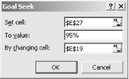
Here is where you can achieve the most extraordinary possible performance leverage without requiring the users to compromise their functional or performance constraints. You've probably heard that SQL tuning offers high payoffs, but it would be nice to know how high before you embark upon a SQL tuning expedition. The model can tell you the answer. If you could, for example, improve the service time of the important statement from 0.49 seconds to 0.3125 seconds, you would improve the service rate for the statement from m = 2.04 stmt/sec to m = 3.2 stmt/sec. If you could improve your service rate just this much, then you could meet the original r max = 1.0 requirement in 95% of statement executions, with just four CPUs. If you could improve average service rate to m = 10 statements per second (for example, by optimizing SQL to reduce average service time to 0.1 seconds), then you could meet the original performance requirements with just one CPU. I believe that the greatest value of the M/M/ m queueing model is that it stimulates you to ask the right questions. In this example, you've learned that it is futile to even think about using more than six CPUs' worth of capacity to run the important statement. You have learned that by negotiating a more liberal r max value with your users, you can gain a little bit of headspace. But until you can reduce either the rate at which people run the important statement ( l ), or reduce the service time of the statement ( S = 1/ m ), you're going to be stuck with a system that at best barely meets its performance target. 9.4.5.5 Using Goal Seek in Microsoft Excel Microsoft Excel provides a Goal Seek tool that makes it simple to answer many of the questions we've discussed in this section. It allows you to treat any model output value as an input parameters. For example, assume that you want to determine what average service rate would be required to drive response time satisfactions into the 95 th percentile for a fixed value of m . You can set up the problem this way. First, enter an arbitrary constant value for m . In Figure 9-24, I have entered the value 1. Next, select the Tools  Goal Seek menu option to activate the goal seek dialog, as shown in Figure 9-25. The goal is to set CDF ( r max ) to the value 95% by changing m . After accepting the result of the goal seek operation, Figure 9-26 shows that using the value m Goal Seek menu option to activate the goal seek dialog, as shown in Figure 9-25. The goal is to set CDF ( r max ) to the value 95% by changing m . After accepting the result of the goal seek operation, Figure 9-26 shows that using the value m  10 produces the desired result. 10 produces the desired result. Figure 9-24. To find what m value we need to drive CDF(r max )  95%, we first enter an arbitrary constant value for 95%, we first enter an arbitrary constant value for Figure 9-25. Our goal is to set CDF(r max ) to the value 95% by changing m  Figure 9-26. After accepting the goal seek solution, our worksheet shows that the value m  10 produces the desired CDF(r max ) value 10 produces the desired CDF(r max ) value  9.4.5.6 Sensitivity analysis The quality of your response time predictions will vary in proportion to the quality of the feedback loop that you use to refine your forecasts. Lots of people get the key numbers right when I present them with a queueing model and ask them to solve a carefully prepared story problem. But you need to resist the temptation to stop thinking, which begins when your model "produces the answer." When the answer comes out, you need to devote a bit more time to the very important task of sensitivity analysis that 99% of people trying models for the first time will habitually fail to do. The remainder of this section illustrates some key points of error analysis for my continuing example. In addition to the model's output, you must consider several other factors: - Physical constraints
-
Of course, it is not possible to install part of a CPU. The number of CPUs you install in a system must be a whole number. Some systems may require a whole number of pairs of CPUs. Physical constraints of course also restrict the maximum number of CPUs that can be installed in a system. - Scalability imperfections
-
The queueing model knows nothing about scalability imperfections that might prevent a system with m CPUs from delivering the full m CPUs' worth of processing capacity. For example, to get six full CPUs' worth of processing from a Linux server, we might need to install eight or more CPUs. Using the Microsoft Windows NT operating system, it might be impossible to configure a system that provides more than two full CPUs' worth of processing capacity, no matter how many CPUs the chassis might accept. It is up to the performance analyst to determine the impact of scalability imperfections that prevent a real m -CPU system from actually delivering m CPU's worth of system capacity. - Other workload
-
Although the problem statement mentioned only a single SQL statement, the system will almost certainly require the execution of several other workload components. Thus, the way to interpret this model's output for this particular problem statement is to conclude that, "The processing capacity required to support the response time requirements of this SQL statement is about 5 more than the number of CPUs required to support all the other load on the system." - Other bottlenecks
-
The problem statement focuses our attention exclusively upon the CPU capacity required to fulfill our response time expectations. But what about other potential bottlenecks? What if our SQL statement's total response time is impacted materially by disk or network latencies? While it is possible to model every resource that participates in a given function, minimizing the complexity of the model often maximizes the model's usefulness . If any resource other than CPU is expected to consume the bulk of a function's response time, then it is reasonable to inquire whether the reason is legitimate. - Changes in input parameters
-
In school, students are often encouraged to believe the assumptions set forth in a neatly packaged problem statement. Successful professionals quickly learn that errors in problem statements account for significant proportions of subsequent project flaws. How can we protect our project from the untrustworthy assumptions documented in the project plan? By assessing the impact of assumption variances upon our model. What is the impact upon our result if one or more of the assumptions laid out in the problem statement is inaccurate or is simply bound to evolve over time? Overall system performance is very sensitive to even very small variances in average service rate ( m ) and average arrival rate ( l ). The model reflects this. The very property that endows these parameters with such leverage upon overall performance makes the model highly susceptible to errors in estimating them. For example, overestimating a function's average service rate by just 1% can result in a 10% or worse underestimate in a loaded system's average response times. Factors that are likely to cause variances in m or l include: -
Invalid testing. Classic examples include tests presumably designed to emulate production database behavior, but which are conducted using unrealistically simple product setups or unrealistically miniscule table sizes. -
Changes in data volume, especially for SQL queries whose performance scales linearly (or worse) to the sizes of the segments being queried [Millsap (2001a)]. -
Changes in physical data distribution that might make an index become more or less useful (or attractive to the Oracle query optimizer) over time [Millsap (2002)]. -
Changes to function code path, such as SQL changes or schema changes motivated by upgrades, performance improvement projects, and so on. -
Changes in business function volume motivated by acquisitions or mergers, unanticipated successes or failures in marketing projects, and so on. If uncontrolled variances in sensitive input parameters are likely, then you should take special care to ensure that the system configuration you choose will permit inexpensive capacity upgrades (or downgrades). With knowledge of input parameter sensitivity, you will know which input parameters to manage the most carefully.
 | | | | |
 /FCFS, which completely describes all five criteria:
  /FCFS (exponential interarrival time)
  /FCFS (exponential service time)
  /FCFS ( m homogeneous, parallel, independent service channels)
  /FCFS (no queue length restriction)
  / FCFS (first-come, first- served queue discipline)
  , and FCFS criteria of the M/M/ m /
  /FCFS model. But it is less clear without further analysis whether the examples meet the M/M criteria. In the next section, we shall explore what it means to say that a random variable is exponentially distributed.
  /FCFS criteria of queueing systems fail to meet the M/M criteria because their arrival and service processes don't fit the exponential distribution. In the next sections, I shall reveal how to test your operational data for fit to the exponential distribution.
 ![]()


 0.8 and that the knee in the bottom curve occurs to the right of
  R /
R / 


 95%, we first enter an arbitrary constant value for