Section 7.3. Copying Formulas
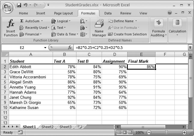
7.3. Copying FormulasSometimes you need to perform similar calculations in different cells throughout a worksheet. For example, say you want to calculate sales tax on each item in a product catalog, the monthly sales in each store of a company, or the final grade for each student in a class. In this section, you'll learn how Excel makes it easy with relative cell references . Relative cell references are cell references that Excel updates automatically when you copy them from one cell into another. They're the standard kind of references that Excel uses (as opposed to absolute cell references, which are covered in the next section). In fact, all the references you've used so far have been relative references, but you haven't yet seen how they work with copy-and-paste operations. Consider the worksheet shown in Figure 7-11, which contains a teacher's grade book. In this example, each student has three grades: two tests and one assignment. A student's final grade is based on the following percentages: 25 percent for each of the two tests, and 50 percent for the assignment.
The following formula calculates the final grade for the first student (Edith Abbott): =B2*25% + C2*25% + D2*50% The formula that calculates the final mark for the second student (Grace DeWitt) is almost identical. The only change is that all the cell references are offset by one row, so that B2 becomes B3, C2 becomes C3, and D2 becomes D3: =B3*25% + C3*25% + D3*50% You may get fed up entering all these formulas by hand. A far easier approach is to copy the formula from one cell to another. Here's how:
Tip: There's an even quicker way to copy a formula to multiple cells by using the AutoFill feature introduced in Chapter 2. In the student grade example, you'd start by moving to cell E2, which contains the original formula. Then, you'd click the small square at the bottom-right corner of the cell outline, and drag the outline down until it covers all cells from E3 to E10. When you release the mouse button, Excel inserts the formula copies in the AutoFill region. 7.3.1. Absolute Cell ReferencesRelative references are a true convenience since they let you create formula copies that don't need the slightest bit of editing. But you've probably already realized that relative references don't always work. For example, what if you have a value in a specific cell that you want to use in multiple calculations? You may have a currency conversion ratio that you want to use in a list of expenses. Each item in the list needs to use the same cell to perform the conversion correctly. But if you make copies of the formula using relative cell references, then you'll find that Excel adjusts this reference automatically and the formula ends up referring to the wrong cell (and therefore the wrong conversion value).
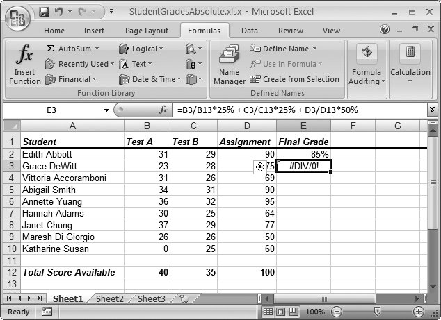
Figure 7-13 illustrates the problem with the worksheet of student grades. In this example, the test and assignment scores aren't all graded out of 100 possible points; each item has a different total score available (listed in row 12). In order to calculate the percentage a student earned on a test, you need to divide the test score by the total score available. This formula, for example, calculates the percentage for Edith Abbott's performance on Test B: =B2/B12*100% To calculate Edith's final grade for the class, you'd use the following formula: =B2/B12*25% + C2/C12*25% + D2/D12*50%
Like many formulas, this one contains a mix of cells that should be relative (the individual scores in cells B2, C2, and D2) and those that should be absolute (the possible totals in cell B12, C12, and D12). As you copy this formula to subsequent rows, Excel incorrectly changes all the cell references, causing a calculation error. Fortunately, Excel provides a perfect solution. It lets you use absolute cell references cell references that always refer to the same cell. When you create a copy of a formula that contains an absolute cell reference, Excel doesn't change the reference (as it does when you use relative cell references; see the previous section). To indicate that a cell reference is absolute, use the dollar sign ($) character. For example, to change B12 into an absolute reference, you would add the $ character twice, once in front of the column and once in front of the row, which changes it to $B$12. Here's the corrected class grade formula (for Edith) using absolute cell references: =B2/$B*25% + C2/$C*25% + D2/$D*50% This formula still produces the same result for the first student. However, you can now copy it correctly for use with the other students. To copy this formula into all the cells in column E, use the same procedure described in the previous section on relative cell references.
7.3.2. Partially Fixed ReferencesYou might wonder why you need to use the $ character twice in an absolute reference (before the column letter and the row number). The reason is that Excel lets you create partially fixed references. To understand partially fixed references, it helps to remember that every cell reference consists of a column letter and a row number. With a partial fixed reference, Excel updates one component (say, the column part) but not the other (the row) when you copy the formula. If this sounds complex (or a little bizarre), consider a few examples:
Tip: You can quickly change formula references into absolute or partially fixed references. Just put the cell into edit mode (by double-clicking it or pressing F2). Then, move through the formula until you've highlighted the appropriate cell reference. Now, press F4 to change the cell reference. Each time you press F4, the reference changes. If the reference is A1, for instance, it becomes $A$1, then A$1, then $A1, and then A1 again.
|
 Clipboard
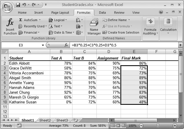
EAN: N/A
Pages: 75