Section 8.2. External Polling
8.2. External PollingIt is often impossible to poll a device internally, for technical, security, or political reasons. For example, the System Administration group may not be in the habit of giving out the root password, making it difficult for you to install and maintain internal polling scripts. However, they may have no problem with installing and maintaining an SNMP agent such as Concord's SystemEDGE or Net-SNMP. It's also possible that you will find yourself in an environment in which you lack the knowledge to build the tools necessary to poll internally. Despite the situation, if an SNMP agent is present on a machine that has objects worth polling, you can use an external device to poll the machine and read the objects' values.[*] This external device can be one or more NMSs or other machines or devices. For instance, when you have a decent-size network, it is sometimes convenient, and possibly necessary, to distribute polling among several NMSs.
Each of the external polling engines we will look at uses the same polling methods, although some NMSs implement external polling differently. We'll start with the OpenView xnmgraph program, which can be used to collect and display data graphically. You can even use OpenView to save the data for later retrieval and analysis. We'll include some examples that show how you can collect data and store it automatically and how you can retrieve that data for display. Castle Rock's SNMPc also has an excellent data-collection facility that we will use to collect and graph data. 8.2.1. Collecting and Displaying Data with OpenViewOne of the easiest ways to get some interesting graphs with OpenView is to use the xnmgraph program. You can run xnmgraph from the command line and from some of NNM's menus. One practical way to graph is to use OpenView's xnmbrowser to collect some data and then click Graph. It's as easy as that. If the node you are polling has more than one instance (say, multiple interfaces), OpenView will graph all known instances. When an NMS queries a device such as a router, it determines how many instances are in the ifTable and retrieves management data for each entry in the table. 8.2.2. OpenView GraphingFigure 8-3 shows the sort of graph you can create with NNM. To create this graph, we started the browser (Figure 8-2) and clicked down through the MIB tree until we found the .iso.org.dod.internet.mgmt.mib-2.interfaces.ifTable.ifEntry list. Once there, we clicked on ifInOctets; then, while holding down the Ctrl key, we clicked on ifOutOctets. After both were selected and we verified that the Name or IP Address field displayed the node we wanted to poll, we clicked on the Graph button. Once the graph has started, you can change the polling interval and the colors used to display different objects. You can also turn off the display of some or all of the object instances. The menu item View Figure 8-3. OpenView xnmgraph of octets in/out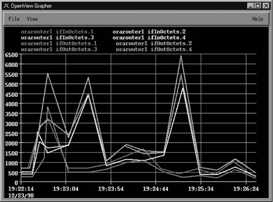 option (View Figure 8-4. xnmgraph statistics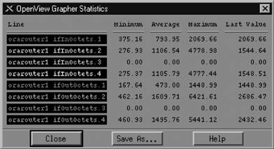
Some of NNM's default menus let you use the grapher to poll devices depending on their type. For example, you can select the object type "router" on the NNM and generate a graph that includes all your routers. Whether you start from the command line or from the menu, sometimes you will get a message back that reads "Requesting more lines than number of colors (25). Reducing number of lines." This message means that there aren't enough colors available to display the objects you are trying to graph. The only good ways to avoid this problem are to break up your graphs so that they poll fewer objects, or eliminate object instances you don't want. For example, you probably don't want to graph router interfaces that are down (for whatever reason) and other "dead" objects. We will soon see how you can use a regular expression as one of the arguments to the xnmgraph command to graph only those interfaces that are up and running. Although the graphical interface is very convenient, the command-line interface gives you much more flexibility. The following shell script displays the graph in Figure 8-3 (i.e., the graph we generated through the browser): #!/bin/sh # filename: /opt/OV/local/scripts/graphOctets # syntax: graphOctets <hostname> /opt/OV/bin/xnmgraph -c public -mib \ ".iso.org.dod.internet.mgmt.mib-2.interfaces.ifTable.ifEntry.ifInOctets::::::::,\ .iso.org.dod.internet.mgmt.mib-2.interfaces.ifTable.ifEntry.ifOutOctets::::::::" \ $1 You can run this script with the command: $ /opt/OV/local/scripts/graphOctets orarouter1 The worst part of writing the script is figuring out what command-line options you wantparticularly the long strings of nine colon-separated options. All these options give you the ability to refine what you want to graph, how often you want to poll the objects, and how you want to display the data. (We'll discuss the syntax of these options as we go along, but for the complete story, see the xnmgraph(1) manpage.) In this script, we're graphing the values of two MIB objects, ifInOctets and ifOutOctets. Each OID we want to graph is the first (and in this case, the only) option in the string of colon-separated options. On our network, this command produces eight traces: input and output octets for each of our four interfaces. You can add other OIDs to the graph by adding sets of options, but at some point, the graph will become too confusing to be useful. It will take some experimenting to use the xnmgraph command efficiently, but once you learn how to generate useful graphs you'll wonder how you ever got along without it.
Now, let's modify the script to include more reasonable labelsin particular, we'd like the graph to show which interface is which, instead of just showing the index number. In our modified script, we've used numerical object IDs, mostly for formatting convenience, and we've added a sixth option to the ugly sequence of colon-separated options: .1.3.6.1.2.1.2.2.1.2 (this is the ifDescr, or interface description, object in the interface table). This option says to poll each instance and use the return value of snmpget .1.3.6.1.2.1.2.2.1.2.INSTANCE as the label. This should give us meaningful labels. Here's the new script: #!/bin/sh # filename: /opt/OV/local/scripts/graphOctets # syntax: graphOctets <hostname> /opt/OV/bin/xnmgraph -c public -title Bits_In_n_Out -mib \ ".1.3.6.1.4.1.9.2.2.1.1.6:::::.1.3.6.1.2.1.2.2.1.2:::,\ .1.3.6.1.4.1.9.2.2.1.1.8:::::.1.3.6.1.2.1.2.2.1.2:::" $1 To see what we'll get for labels, here's the result of walking .1.3.6.1.2.1.2.2.1.2: $ snmpwalk orarouter1 .1.3.6.1.2.1.2.2.1.2 interfaces.ifTable.ifEntry.ifDescr.1 : DISPLAY STRING- (ascii): Ethernet0 interfaces.ifTable.ifEntry.ifDescr.2 : DISPLAY STRING- (ascii): Serial0 interfaces.ifTable.ifEntry.ifDescr.3 : DISPLAY STRING- (ascii): Serial1 Figure 8-5 shows our new graph. With the addition of this sixth option, the names and labels are much easier to read. Meaningful labels and titles are important, especially if management is interested in seeing the graphs. A label that contains an OID and not a textual description is of no use. Some objects that are useful in building labels are ifType (.1.3.6.1.2.1.2.2.1.3) and ifOperStatus (.1.3.6.1.2.1.2.2.1.8). Be careful when using ifOperStatus; if the status of the interface changes during a poll, the label does not change. The label is evaluated only once. One of the most wasteful things you can do is poll a useless object. This often happens when an interface is administratively down or not configured. Imagine that you Figure 8-5. OpenView xnmgraph with new labels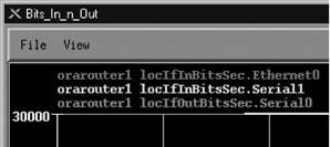 have 20 serial interfaces, but only one is actually in use. If you are looking for octets in and out of your serial interfaces, you'll be polling 40 times and 38 of the polls will always read 0. OpenView's xnmgraph allows you to specify an OID and regular expression to select what should be graphed. To put this feature to use, let's walk the MIB to see what information is available: $ snmpwalk orarouter1 .1.3.6.1.2.1.2.2.1.8 interfaces.ifTable.ifEntry.ifOperStatus.1 : INTEGER: up interfaces.ifTable.ifEntry.ifOperStatus.2 : INTEGER: up interfaces.ifTable.ifEntry.ifOperStatus.3 : INTEGER: down This tells us that only two interfaces are currently up. By looking at ifDescr, we see that the live interfaces are Ethernet0 and Serial0; Serial1 is down. Notice that the type of ifOperStatus is INTEGER, but the return value looks like a string. How is this? RFC 1213 defines string values for each possible return value: ifOperStatus OBJECT-TYPE SYNTAX INTEGER { up(1), --ready to pass packets down(2), testing(3) --in some test mode } ACCESS read-only STATUS mandatory DESCRIPTION "The current operational state of the interface. The testing(3) state indicates that no operational packets can be passed." ::= { ifEntry 8 } It's fairly obvious how to read this: the integer value 1 is converted to the string up. We can therefore use the value 1 in a regular expression that tests ifOperStatus. For every instance we will check the value of ifOperStatus; we will poll that instance and graph the result only if the status returns 1. In pseudocode, the operation would look something like this: if (ifOperStatus == 1) { pollForMIBData; graphOctets; } Here's the next version of our graphing script. To put this logic into a graph, we use the OID for ifOperStatus as the fourth colon option and the regular expression (1) as the fifth option: #!/bin/sh # filename: /opt/OV/local/scripts/graphOctets # syntax: graphOctets <hostname> /opt/OV/bin/xnmgraph -c public \ -title Octets_In_and_Out_For_All_Up_Interfaces \ -mib ".1.3.6.1.2.1.2.2.1.10:::.1.3.6.1.2.1.2.2.1.8:1::::, \ .1.3.6.1.2.1.2.2.1.16:::.1.3.6.1.2.1.2.2.1.8:1::::" $1 This command graphs the ifInOctets and ifOutOctets of any interface that has a current operational state equal to 1, or up. It therefore polls and graphs only the ports that are important, saving on network bandwidth and simplifying the graph. Furthermore, we're less likely to run out of colors while making the graph because we won't assign them to useless objects. Note, however, that this selection happens only during the first poll and stays effective throughout the entire life of the graphing process. If the status of any interface changes after the graph has been started, nothing in the graph will change. The only way to discover any changes in interface status is to restart xnmgraph. Finally, let's look at:
The cropped graph in Figure 8-6 shows how the labels change when we run the following script: #!/bin/sh # filename: /opt/OV/local/scripts/graphOctets # syntax: graphOctets <hostname> /opt/OV/bin/xnmgraph -c public -title Internet_Traffic_In_K -poll 68 -mib \ ".1.3.6.1.4.1.9.2.2.1.1.6:Incoming_Traffic::::.1.3.6.1.2.1.2.2.1.2::.001:,\ .1.3.6.1.4.1.9.2.2.1.1.8:Outgoing_Traffic::::.1.3.6.1.2.1.2.2.1.2::.001:" \ $1 The labels are given by the second and sixth fields in the colon-separated options (the second field provides a textual label to identify the objects we're graphing and the sixth uses the ifDescr field to identify the particular interface); the constant multiplier (.001) is given by the eighth field; and the polling interval (in seconds) is given by the -poll option. By now it should be apparent how flexible OpenView's xnmgraph program really is. These graphs can be important tools for troubleshooting your network. When a network manager receives complaints from customers regarding slow connections, he can look at the graph of ifInOctets generated by xnmgraph to see if any router interfaces have unusually high traffic spikes. Figure 8-6. xnmgraph with labels and multipliers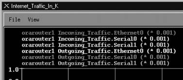 Graphs like these are also useful when you're setting thresholds for alarms and other kinds of traps. The last thing you want is a threshold that is too "triggery" (one that goes off too many times) or a threshold that won't go off until the entire building burns to the ground. It's often useful to look at a few graphs to get a feel for your network's behavior before you start setting any thresholds. These graphs will give you a baseline from which to work. For example, say you want to be notified when the battery on your UPS is low (which means it is being used) and when it is back to normal (fully charged). The obvious way to implement this is to generate an alarm when the battery falls below some percentage of full charge, and another alarm when it returns to full charge. So the question is: what value can we set for the threshold? Should we use 10% to indicate that the battery is being used and 100% to indicate that it's back to normal? We can find the baseline by graphing the device's MIBs.[*] For example, with a few days' worth of graphs, we can see that our UPS's battery stays right around 94-97% when it is not in use. There was a brief period where the battery dropped down to 89% when it was performing a self-test. Based on these numbers, we may want to set the "in use" threshold at 85% and the "back to normal" threshold at 94%. This pair of thresholds gives us plenty of notification when the battery's in use but won't generate useless alarms when the device is in self-test mode. The appropriate thresholds depend on the type of devices you are polling, as well as the MIB data that is gathered. Doing some initial testing and polling to get a baseline (normal numbers) will help you set thresholds that are meaningful and useful.
Before leaving xnmgraph, we'll take a final look at the nastiest aspect of this program: the sequence of nine colon-separated options. In the examples, we've demonstrated the most useful combinations of options. In more detail, here's the syntax of the graph specification: object:label:instances:match:expression:instance-label:truncator:multiplier:nodes The parameters are:
The only required field is object; however, as we've seen, you must have all eight colons even if you leave some (or most) of the fields empty. 8.2.3. OpenView Data Collection and ThresholdsOnce you close the OpenView graphs, the data in them is lost forever. OpenView provides a way to fix this problem with data collection. Data collection allows the user to poll and record data continuously. It can also look at these results and trigger events. One benefit of data collection is that it can watch the network for you while you're not there; you can start collecting data on Friday and then leave for the weekend, knowing that any important events will be recorded in your absence. You can start OpenView's Data Collection and Thresholds function from the command line, using the command $OV_BIN/xnmcollect, or from NNM under the Options menu. This brings you to the Data Collection and Thresholds window, shown in Figure 8-7, which displays a list of all the collections you have configured and a summary of the collection parameters. Figure 8-7. OpenView's Data Collection and Thresholds window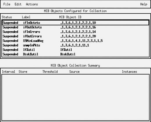 Configured collections that are in Suspended mode appear in a dark or bold font. This indicates that OpenView is not collecting any data for these objects. A Collecting status indicates that OpenView is polling the selected nodes for the given object and saving the data. To change the status of a collection, select the object, click on Actions, and then click on either Suspend Collection or Resume Collection. (Note that you must save your changes before they will take effect.) 8.2.3.1. Designing collectionsTo design a new collection, select Edit .iso.org.dod.internet.private.enterprises.hp.nm.system.net-peripheral.net-printer.generalDeviceStatus.gdStatusEntry.gdStatusPaperOut (.1.3.6.1.4.1.11.2.3.9.1.1.2.8).[*]
The object's description suggests that this is the item we want: it reads "This indicates that the peripheral is out of paper." (If you already know what you're looking for, you can enter the name or OID directly.) Once there, you can change the name of the collection to something that is easier to read. Click OK to move forward. This brings you to the menu shown in Figure 8-8. The Source field is where you specify the nodes from which you would like to collect data. Enter the hostnames or IP addresses you want to poll. You can use wildcards like 198.27.6.* in your IP addresses; you can also click Add Map to add any nodes currently selected. We suggest that you start with one node for testing purposes. Adding more nodes to a collection is easy once you have everything set up correctly; you just return to the window in Figure 8-8 and add the nodes to the Source list. Collection Mode lets you specify what to do with the data NNM collects. There are four collection modes: Exclude Collection; Store, Check Thresholds; Store, No Thresholds; and Don't Store, Check Thresholds. Except for Exclude Collection, which allows us to turn off individual collections for each device, the collection modes are fairly self-explanatory. (Exclude Collection may sound odd, but it is very useful if you want to exclude some devices from data collection without stopping the entire process; for example, you may have a router with a hardware problem that is bombarding you with meaningless data.) Data collection without a threshold is easier than collection with a threshold, so we'll start there. Set the Collection Mode to Store, No Thresholds. This disables (grays out) the bottom part of the menu, which is used for threshold parameters. (Select Store, Check Thresholds if you want both data collection and threshold monitoring.) Then click OK and save the new collection. You can now watch your collection grow in the $OV_DB/snmpCollect directory. Each collection consists of a binary datafile, plus a file with the same name Figure 8-8. OpenView poll configuration menu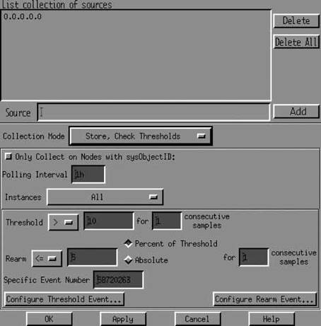 preceded by an exclamation mark (!); this file stores the collection information. The data collection files will grow without bounds. To trim these files without disturbing the collector, delete all files that do not contain an ! mark. Clicking on Only Collect on Nodes with sysObjectID allows you to enter a value for sysObjectID. sysObjectID (iso.org.dod.internet.mgmt.mib-2.system.sysObjectID) lets you limit polling to devices made by a specific manufacturer. Its value is the enterprise number the device's manufacturer has registered with IANA. For example, Cisco's enterprise number is 9, and HP's is 11 (the complete list is available at http://www.iana.org/assignments/enterprise-numbers); therefore, to restrict polling to devices manufactured by HP, set the sysObjectID to 11. RFC 1213 formally defines sysObjectID (1.3.6.1.2.1.1.2) as follows: sysObjectID OBJECT-TYPE SYNTAX OBJECT IDENTIFIER ACCESS read-only STATUS mandatory DESCRIPTION "The vendor's authoritative identification of the network management subsystem contained in the entity. This value is allocated within the SMI enterprises subtree (1.3.6.1.4.1) and provides an easy and unambiguous means for determining what kind of box' is being managed. For example, if vendor 'Flintstones, Inc.' was assigned the subtree 1.3.6.1.4.1.4242, it could assign the identifier 1.3.6.1.4.1.4242.1.1 to its 'Fred Router'." ::= { system 2 } The polling interval is the period at which polling occurs. You can use one-letter abbreviations to specify units: s for seconds, m for minutes, h for hours, and d for days. For example, 32s indicates 32 seconds; 1.5d indicates one and a half days. When we're designing a data collection, we usually start with a very short polling intervaltypically 7s (7 seconds between each poll). You probably wouldn't want to use a polling interval this short in practice (all the data you collect is going to have to be stored somewhere), but when you're setting up a collection, it's often convenient to use a short polling interval. You don't want to wait a long time to find out whether you're collecting the right data. The next option is a drop-down menu that specifies what instances should be polled. The options are All, From List, and From Regular Expression. In this case, we're polling a scalar item, so we don't have to worry about instances; we can leave the setting to All or select From List and specify instance 0 (the instance number for all scalar objects). If you're polling a tabular object, you can either specify a comma-separated list of instances or choose the From Regular Expression option and write a regular expression that selects the instances you want. Save your changes (File 8.2.3.2. Creating a thresholdOnce you've set all this up, you've configured NNM to periodically collect the status of your printer's paper tray. Now for something more interesting: let's use thresholds to generate some sort of notification when the traffic coming in through one of our network interfaces exceeds a certain level. To do this, we'll look at a Cisco-specific object, locIfInBitsSec (more formally iso.org.dod.internet.private.enterprises.cisco.local.linterfaces.lifTable.lifEntry.locIfInBitsSec), whose value is the five-minute average of the rate at which data arrives at the interface, in bits per second. (There's a corresponding object called locIfOutBitsSec, which measures the data leaving the interface.) The first part of the process should be familiar: start Data Collection and Thresholds by going to the Options menu of NNM, then select Edit Setting an appropriate consecutive samples value will make your life much more pleasant, though picking the right value is something of an art. Another example is monitoring the /tmp partition of a Unix system. In this case, you may want to set the threshold to >= 85, the number of consecutive samples to 2, and the poll interval to 5m. This will generate an event when the usage on /tmp exceeds 85% for two consecutive polls. This choice of settings means that you won't get a false alarm if a user copies a large file to /tmp and then deletes the file a few minutes later. If you set consecutive samples to 1, NNM generates a Threshold event as soon as it notices that /tmp is filling up, even if the condition is only temporary and nothing to be concerned about. It then generates a Rearm event after the user deletes the file. Since we are really only worried about /tmp filling up and staying full, setting the consecutive threshold to 2 can help reduce the number of false alarms. This is generally a good starting value for consecutive samples, unless your polling interval is very high. The rearm parameters let us specify when everything is back to normal or is, at the very least, starting to return to normal. This state must occur before another threshold is met. You can specify either an absolute value or a percentage. When monitoring the packets arriving at an interface, you might want to set the rearm threshold to something like 926,400 bits per second (an absolute value that happens to be 60% of the total capacity) or 80% of the threshold (also 60% of capacity). Likewise, if you're generating an alarm when /tmp exceeds 85% of capacity, you might want to rearm when the free space returns to 80% of your 85% threshold (68% of capacity). You can also specify the number of consecutive samples that need to fall below the rearm point before NNM considers the rearm condition met. The final option, Configure Threshold Event, asks what OpenView events you would like to execute for each state. You can leave the default event, or you can refer to Chapter 9 for more on how to configure events. The Threshold state needs a specific event number that must reside in the HP enterprise. The default Threshold event is OV_DataCollectThresh - 58720263. Note that the Threshold event is always an odd number. The Rearm event is the next number after the Threshold event: in this case, 58720264. To configure events other than the default, click on Configure Threshold Event and, when the new menu comes up, add one event (with an odd number) to the HP section and a second event for the corresponding Rearm. After making the additions, save and return to the Collection window to enter the new number. When you finish configuring the data collection, click OK. This brings you back to the Data Collection and Thresholds menu. Select File Once you have collected some data, you can use xnmgraph to display it. The xnmgraph command to use is similar to the ones we saw earlier; it's an awkward command that you'll want to save in a script. In the following script, the -browse option points the grapher at the stored data: #!/bin/sh # filename: /opt/OV/local/scripts/graphSavedData # syntax: graphSavedData <hostname> /opt/OV/bin/xnmgraph -c public -title Bits_In_n_Out_For_All_Up_Interfaces \ -browse -mib \ ".1.3.6.1.4.1.9.2.2.1.1.6:::.1.3.6.1.2.1.2.2.1.8:1:.1.3.6.1.2.1.2.2.1.2:::,\ .1.3.6.1.4.1.9.2.2.1.1.8:::.1.3.6.1.2.1.2.2.1.8:1:.1.3.6.1.2.1.2.2.1.2:::" \ $1 Once the graph has started, no real (live) data is graphed; the display is limited to the data that has been collected. You can select File Finally, to graph all the data that has been collected for a specific node, go to NNM and select the node you would like to investigate. Then select Performance 8.2.4. Castle Rock's SNMPcThe workgroup edition of Castle Rock's SNMPc program has similar capabilities to the OpenView package. It uses the term trend reporting for its data collection and threshold facilities. The enterprise edition of SNMPc even allows you to export data to a web page. To see how SNMPc works, let's graph the snmpOutPkts object. This object's OID is 1.3.6.1.2.1.11.2 (iso.org.dod.internet.mgmt.mib-2.snmp.snmpOutPkts). It is defined in RFC 1213 as follows: snmpOutPkts OBJECT-TYPE SYNTAX Counter ACCESS read-only STATUS mandatory DESCRIPTION "The total number of SNMP messages which were passed from the SNMP protocol entity to the transport service." ::= { snmp 2 } We'll use the orahub device for this example. Start by clicking on the MIB Database selection tab shown in Figure 8-9; this is the tab at the bottom of the screen that looks something like a spreadsheetit's the second from the left. Click down the tree until you come to iso.org.dod.internet.mgmt.mib-2.snmp. Click on the object you would like to graph (for this example, snmpOutPkts). You can select multiple objects with the Ctrl key. Figure 8-9. SNMPc MIB Database view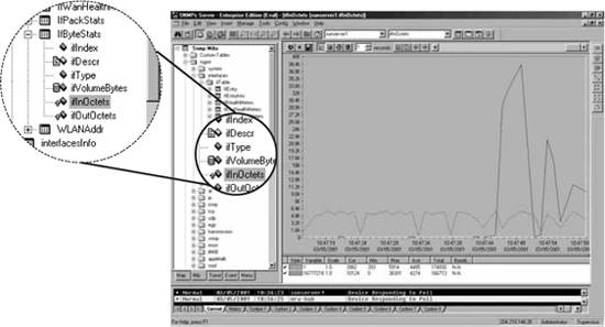
Once you have selected the appropriate MIB object, return to the top level of your map by either selecting the house icon or clicking on the Root Subnet tab (at the far left) to select the device you would like to poll. Instead of finding and clicking on the device, you can enter the device's name by hand. If you have previously polled the device, you can select it from the drop-down box. Figure 8-10 shows what a completed menu bar should look like. Figure 8-10. SNMPc menu bar graph section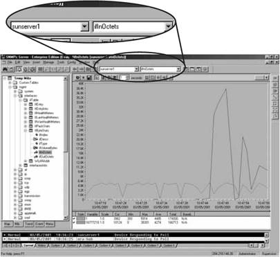 To begin graphing, click the button with the small jagged graph (the third from the right). Another window will appear displaying the graph (Figure 8-11). The controls at the top change the type of graph (line, bar, pie, distribution, etc.) and the polling interval and allow you to view historical data (the horizontal slider bar). Review the documentation on how each of these work or, better yet, play around to learn these menus even faster. Once you have a collection of frequently used graphs, you can insert them into the custom menus. Let's insert a menu item in the Tools menu that displays all the information in the snmpInfo table as a pie chart. Click on the Custom Menus tab (the last one), right-click on the Tools folder, and then left-click on Insert Menu. This gets you to the Add Custom Menu window (Figure 8-12). Enter a menu name and select Pie for the display type. Use the browse button (>>) to click down the tree of MIB objects until you reach the snmpInfo table and click OK. Back at Add Custom Menu, use the checkboxes in the Use Selected Object section to specify the types of nodes that will be able to respond to this custom menu item. For example, to chart snmp- Figure 8-11. SNMPc snmpOutPkts graph section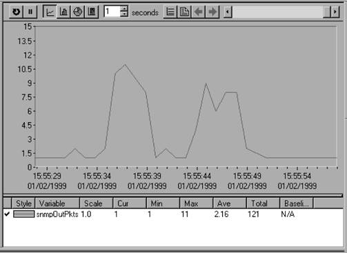 Info, a device obviously needs to support SNMP, so we've checked the Has SNMP box. This information is used when you (or some other user) try to generate this chart for a given device. If the device doesn't support the necessary protocols, the menu entry for the pie chart will be disabled. Figure 8-12. SNMPc Add Custom Menu window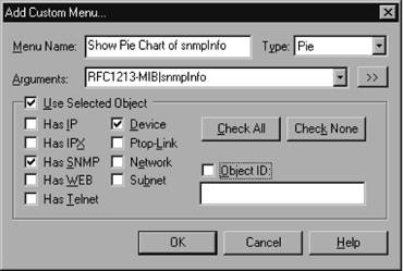 Click OK and proceed to your map to find a device to test. Any SNMP-compatible device should suffice. Once you have selected a device, click on Tools and then Show Pie Chart of snmpInfo. You should see a pie chart displaying the data collected from the MIB objects you have configured. (If the device doesn't support SNMP, this option will be disabled.) Alternately, you could have double-clicked your new menu item in the Custom Menu tab. SNMPc has a threshold system called Automatic Alarms that can track the value of an object over time to determine its highs and lows (peaks and troughs) and get a baseline. After it obtains the baseline, it alerts you if something strays out of bounds. In the main menu, selecting Config Figure 8-13. SNMPc Trend Reports Global Settings menu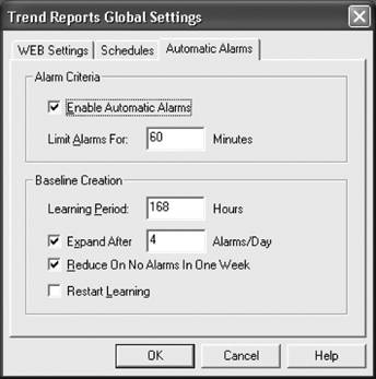 Check the Enable Automatic Alarms box to enable this feature. The Limit Alarms For box lets you specify how much time must pass before you can receive another alarm of the same nature. This prevents you from being flooded by the same message over and over again. The next section, Baseline Creation, lets you configure how the baseline will be learned. The learning period is how long SNMPc should take to figure out what the baseline really is. The Expand After option, if checked, states how many alarms you can get in one day before SNMPc increases the baseline parameters. In Figure 8-13, if we were to get four alarms in one day, SNMPc would increase the threshold to prevent these messages from being generated so frequently. Checking the Reduce On No Alarms In One Week box tells SNMPc to reduce the baseline if we don't receive any alarms in one week. This option prevents the baseline from being set so high that we never receive any alarms. If you check the last option and click OK, SNMPc will restart the learning process. This gives you a way to wipe the slate clean and start over. 8.2.5. Open Source Tools for Data Collection and GraphingOne of the most powerful tools for data collection and graphing is MRTG, familiar to many in the open source community. It collects statistics and generates graphical reports in the form of web pages. In many respects, it's a different kind of animal than the tools discussed in this chapter. RRDtool is the successor to MRTG. Cricket is a popular frontend for RRDtool. We cover MRTG in Chapter 12 and Cricket and RRDtool in Chapter 13. |
 Line Configuration lets you specify which objects you would like to display; it can also set multipliers for different items. For example, to display everything in K, multiply the data by .001. There is also an
 Add MIB Object. This takes you to a new screen. At the top, click on MIB Object[*] You can collect the value of an expression instead of a single MIB object.
EAN: 2147483647
Pages: 165