A Physicist Looks at Project Progress

As luck would have it, I sought refuge in a simple model, that of Newton's Second Law. Because all of classical mechanics is dominated by this simple principle, perhaps there was a "Newton's Second Law" for software development projects. After all, projects tend to have a "percent completion" curve that is remarkably consistent from project to project. Could I attempt to describe the underlying forces acting on the project by considering the derivatives of this curve? While extending the laws of physics to project dynamics may be somewhat speculative, I hoped to help project managers understand the rhythm of their teams.^[1]

^[1] This analysis also appeared in somewhat condensed form in the August 2002 issue of Dr. Dobbs' Journal.

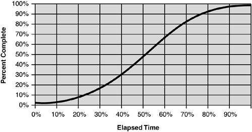
Have You Seen This One Before?

Most of the time, progress curves reported at the end of a project look like the one shown in Figure 12.1.

Figure 12.1. A typical project percent complete curve.

In fact, most projects are planned to have a progress curve that looks like this. Most wind up reporting progress that looks somewhat like the plan, with some distortion to reflect reality.

Because so many project completion curves look like this, I began to wonder if there are fundamental forces at work that cause the curve to be this way.

It All Goes Back to Newton

Some people claim that "modern" physics started with Newton, although the first modern physicist was probably Galileo. What Newton told us in his Second Law was that the acceleration of a body was proportional to the net force applied to it, the proportionality constant being the inverse of its mass.^[2] The more force, the more acceleration.

^[2] By net force, I mean the sum of all the forces acting on the mass. This is most often expressed by the formula F = ma, where F and a are in bold because they are vector quantities. I drop this vector notation to simplify things, as I am generally working in one dimension. Also, note that the more general form of the second law is F = dp/dt, where p is the momentum. This reduces to F = ma if the mass is constant, something I also assume for the rest of the chapter. This is a very crucial assumption; scope creep corresponds to the project becoming more massive, invalidating the analysis. One must constantly guard against increases in scope; even small ones pile up in an insidious fashion.

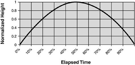
The problem is that acceleration is something we rarely experience. We experience it when our car peels out at a stoplight, when we stomp down on the brakes, or when an elevator first takes off or comes to a sharp stop. More often, we are aware of two other variables: velocity (speed, in common parlance) and position (location, or where we are). We seem to be aware of going fast or going slowly, and we are usually aware of where we are. But force is only indirectly related to these metrics.

Derivatives, Rates of Change, and the Slope of the Tangent

If you are calculus-aware, you know that velocity is the first derivative of position, and that acceleration is the first derivative of velocity, making acceleration the second derivative of position. If you never mastered calculus (or have forgotten it), substitute "rate of change" for "derivative." That is, your velocity is the rate of change of your position, and your acceleration is the rate of change of your velocity.

According to Newton, acceleration is proportional to the net force applied, so the second derivative of the position of an object is proportional to the force. Another way of saying this is that you have to take the net applied force and integrate twice to get information about the position. This is definitely not something that is intuitive for most of us. So I'll leave this integrating twice business alone for now, with the knowledge that there is sufficient mathematics to perform our integrations and differentiations once we understand the mechanisms.

If you reason or think better graphically, remember that you can find the derivative or rate of change for any curve by looking at a line tangent to the curve at the point in which you are interested. For example, in Figure 12.2the parabolathe derivative or rate of change at the midpoint is zero. We can tell this because the tangent line to the curve there is horizontal, which has a slopeor rate of changeof zero. Prior to that, the tangent at any point has a positive slope; after the midpoint, the slope is negative.

Figure 12.2. Trajectory for a vertical ball toss.

A Simple Physical Example

A ball thrown vertically up in the air has a very well-defined trajectory.^[3] If I plot the height as a function of time, I get the nice parabola shown in Figure 12.2.^[4]

^[3] For the purposes of this example, I will ignore air resistance. As in all physics experiments that make this assumption, this has the disastrous side effect of killing the experimenter, as he has no air to breathe.

^[4] A note on the graphs in this chapter: I used Excel to plot them. I took the horizontal axiselapsed timeto run from 0 to 100 percent, and then I used mathematical formulae to generate the data values. I always normalize the vertical axis to "one"that is, I have the height go from zero to its maximum, which I call "one." I computed all the derivatives numerically, once again using Excel to do the computations and the plots. Hence, you can replicate all of this yourself and need no knowledge of calculus to derive the results.

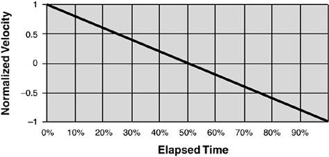
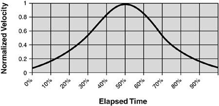
Now if I plot the velocity of the ball,^[5] I get the graph shown in Figure 12.3.

^[5] I do this by numerically differentiating the data points from the parabolic curve. That is, I take successive differences of the values of the first curve, then multiply by a constant to get the values to fall between plus and minus one. The careful observer will notice that this causes us to "miss" the first point on the first derivative curve, and the first two points on the second derivative curve, and also causes a very slight shift (half a bin, actually) on the derivative curves. This won't become noticeable until later; it doesn't affect the arguments at all, but is just an artifact of how I am computing the derivatives.

Figure 12.3. Velocity for a vertical ball toss.

Note that I have "normalized" the vertical axis so that the velocity falls between plus one and minus one; this helps us understand the concept by abstracting out the numbers.^[6] This graph tells us that the ball starts out with a maximum velocity of one "unit," and that velocity decreases linearly until its reaches zero at the midpoint of its flight. This makes sense to us, because the midpoint of the flight is the highest point it achieves; at that instant, the ball is going neither up nor down, so its velocity is zero. Then it begins to fall, so its velocity is negative.^[7] When the ball arrives at its starting point, its speed is exactly the same as when it was launched, except it is moving in the opposite direction.

^[6] One convention is important: the "up" direction is positive. This will determine which velocities are positive and negative.

^[7] Hence the difference between velocity and speed. Speed is always positive; as the ball falls, it speeds up. However, its velocity becomes more negative. The number representing speed and velocity gets larger in magnitude; however, velocity takes into account direction, so it becomes a larger negative number.

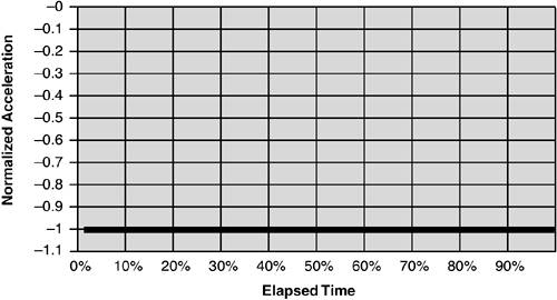
Now, what about acceleration? Well, I just repeat the process one more time, obtaining the graph shown in Figure 12.4.

Figure 12.4. Acceleration for a vertical ball toss.

Once again, I have "normalized" the numerical value to -1.^[8] What this is telling us is that there is a constant acceleration. That is consistent with our model; close to the surface of the earth, the gravitational force is constant. And it is "negative" because I have chosen "up" to be positive, so the attractive force of gravity pulls the ball "down."

^[8] Our friend Excel insists on calling zero "-0." We are smart enough to know that there is only one zero, and it doesn't have a sign.

Note that this acceleration is negative for the entire flight of the balleven when the velocity is positive (upward flight), the acceleration is negative. We are "subtracting" velocity throughout the flight: We start out with some positive velocity which reduces to zero at the highest point, and then we keep subtracting until the velocity is as negative at the end as it was positive at the beginning.

Whew! Newton is vindicated. I have "experimentally" verified that a parabolic position graph implies a constant acceleration, which in turn implies a constant (gravitational) force.

Can I use reasoning of this type to understand the "forces" at work on a project? As with acceleration, we do not experience these forces directly. Rather, we observe things that are indirectly related. So let's return to the percent complete curve; it describes what happened, plotting the combined results of all those forces we don't directly observe. If we assume this project completion graph is prototypical, then what would that tell us about project dynamics?

The "Project Completion" Graph: Plotting Position Against Time

As I have already pointed out, most projects can be plotted according to Figure 12.1.^[9] Note that I have once again normalized things, so that the time axis goes from 0 to 100 percent, and the vertical axis also goes from 0 to 100 percent. Also note that I have somewhat arbitrarily positioned 50 percent complete at 50 percent of the elapsed time. The symmetry of the curve is a simplifying assumption, but one that is useful for this exposition. For the time being, I have no reason to assume otherwise.^[10]

^[9] Here come the caveats. This is of course an idealization. Real-life curves are rarely so smooth. Also, projects don't uniformly move forward, although it is rare to see a reported percent completion curve show a dip. But the real problem is that there is no single metric we can use across the entire project to capture "percent complete." One of the largest problems on any project is figuring out how to distinguish reported progress from actual progress.

^[10] You may see curves that look like this that have various other "percent completes" at 50 percent of the elapsed time. It is allowed. I don't deal with them here for simplicity.

The Curve of Human Behavior

Generically, these curves are referred to as S-curves because they resemble the letter S if you stand back a bit and squint. They describe a wide variety of human behavior; the classic "learning curve," for instance, assumes this shape. The notion that a project completion curve mirrors a learning curve ought to tell us something.

When we begin to learn something new, we spend a lot of time fumbling around without understanding much. This corresponds to the first, flat part of the curve, where time goes by without much progress. Then, as we begin to understand what is going on, our progress increases; this is reflected by the second part of the curve, sometimes called the ramp. During this period we actually make a lot of progress per unit time, and if we could continue at this rate we would finish our task sooner. But inevitably, we enter the third part of the curve, which goes flat on us again. What is happening here is that we plateau; we stop making dramatic progress, and the last few percent (learning all those remaining annoying details) takes a long time. This learning experience is repeatable over and over again, from domain to domain.

When the ramp is gently inclined, we talk about an easy learning curve; when the ramp goes up very fast, we talk about a steep learning curve. Many people cannot handle steep learning curves; they need more time to assimilate the bulk of the new knowledge.

Quick studies are interesting people; they have a very short approach period, go up a very steep ramp, and then quit without ever learning the last few percent. By truncating both flat parts and navigating steep ramps, they can radically abbreviate the time it takes them to acquire knowledge and skills. But they are rare indeed. Most of us do best with two flat parts and a moderate ramp.

Projects follow a similar rhythm. Early in the project, you make progress slowly. There is a lot of planning, organizing, and discovery that causes you to expend a lot of effort without making much tangible progress. Once you get going, you get on the ramp and progress feels (and probably is) somewhat linear (although we know it is not quite linear). Late in the project, things slow down again, which explains why finishing is hard. Once again, nailing down all the details you need to complete to deliver the product takes a relatively long time to do. That is why a project that is 90 percent complete is probably low risk from a technical point of view, but will still take awhile to finish. Things slow down at the end, and there is almost nothing you can do to fix that. Adding people at this stage, for example, will just push the end date further out, as has been shown over and over again.

What about new product acceptance in the marketplace? Same thing. Slow at first, as people have to find out about the product, understand its costs and benefits, talk to their colleagues, and go through a selection and acquisition process. These are the early adopters. Then there is a ramp, when the product "catches on" and demand seems to go through the roof. This is the point Geoffrey Moore calls crossing the chasm, when a product goes mainstream.^[11] This goes on for a while, and then sales begin to slow. We have now hit the third part of the curve: the plateau. The product is now deemed "mature," with trailing or late adopters being the principal buyers. Very likely, another rival product is hitting its ramp at this point and taking away market share from the earlier product. So this universal curve also represents a product's sales lifecycle.

^[11] Moore, Geoffrey A. and Regis McKenna, Crossing the Chasm: Marketing and Selling High-Tech Products to Mainstream Customers, Revised Edition (New York: Harper Business, 1999).

The Project Velocity Curve

Before getting into myriad debates about how "real" this curve is, let's just assume that it represents the majority of reported "percent complete" data and see what can be inferred. Like many other examples in physics, we first try to understand the idealized behavior, and then modify our conclusions by adding back in the effects of air resistance and other real-world phenomena to the model.

The crucial observation is that this curve is a "position versus time" plot. In other words, this curve plots our "position" at any point in time. Now, what does the "velocity" curve look like?

Mimicking the steps used previously, we have the technology to answer that question. Taking the rate of change of our project completion curve yields the graph shown in Figure 12.5.

Figure 12.5. Velocity for project percent complete curve.

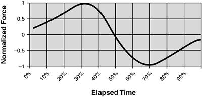
By now you are used to having the vertical axis normalized. What this graph tells us is that projects start off slowly and move faster for a while. Then they reach maximum velocity (in Figure 12.5, maximum velocity is achieved at the halfway point, but that is because our project completion curve is symmetric), and then start to slow down. As you cross the finish line, you are actually going fairly slowly, much as you did at the very beginning.

This is consistent with our common, everyday experience. Projects are slow to get started, they seem to "gather momentum" at some point, and then they "bog down," and things go more slowly. Finishing is hard. Getting all the fine details worked out so that you can deliver the product seems to take forever. Often it feels like you stagger across the finish line.

Once again, the exact values for this curve may vary, but the pattern, from project to project, is remarkably consistent. So what does this say about the underlying "forces" driving the project?

Well, at this point the physicist would take another derivative. Let's do that!

The Project Forces Graph

The resulting acceleration curve, which implies the forces at work, is shown in Figure 12.6.^[12]

^[12] The slight shift mentioned in Footnote 5 is noticeable here; the forces curve should cross the axis at 50 percent. Once again, this is an artifact of the crude way in which I compute the derivative and is absolutely irrelevant to the argument.

Figure 12.6. Net project forces as shown by the acceleration for project percent complete curve.

What are we to make of this?

Well, here's one interpretation: During the first third of the project, we see an increasing positive force. This corresponds to a lot of enthusiasm for the new project, the addition of new team members, and a general optimism about the chances of success. This might cynically be called the "ignorance is bliss period." It is this positive, increasing force that causes the project to gain velocity (sometimes colloquially called momentum, or "the big mo").^[13] At about the one-third point, this positive force begins to decline. This could correspond to reality setting in; people are far enough along to start to understand what the real problems are and are beginning to feel some schedule pressure. After all, they have now used up one-third of the time but still have mountains of work left to do. Also, the team is beginning to feel the full burden of a large staff; a lot of time is spent in meetings, and communicating information to all the members of the team grows difficult.

^[13] Physics seems to intrude into our language even when I don't want it to.

And then we reach the halfway point. At this point, according to the previous graph, a negative force sets in. The team begins to feel the project "pushing back." Many of the really tough problems are not succumbing to solutions as quickly as we thought. People begin to really panic as more and more sand slips through the narrows of the hourglass. At about the two-thirds point, the force hits its maximum negative value; there is this sensation of swimming in molasses. If the project stays here for very long, it dies.

And then, when we most need it, the project "turns the corner." There is a breakthrough, and all of a sudden things don't look quite so bleak anymore.^[14] While there is still a negative force at workthe knowledge that there are still a million details left to complete, and not much time in which to finish themthis negative force decreases. The main reason for this is that the team can see the finish line. The negativity decreases until we get across the finish line.

^[14] The more crusty project manager may be heard to murmur at this juncture, "We may finally have broken the back of this son of a bitch."

Be aware that the actual "turning points" on this curveone-third, one-half, two-thirdswill vary from project to project, and will in turn affect the velocity curve and the project percent completion curve. There is nothing magic about the one-third, one-half, and two-thirds completion points; these result from the symmetric project completion curve I originally chose for ease of exposition. The exact points on our project are unknowable; all we can "predict" is that it will go through these phases.

This is kind of gratifying. I start with a prototypical percent complete curve, take a couple of derivatives, and infer the forces underlying the project. The data seems to empirically fit the theory. Have I really accomplished anything here?