11.2 Supervisor Worker

11.2 Supervisor – Worker

Supervisor – Worker is a concurrent architecture that can be used to speed up the execution of some computational problems by exploiting parallel execution on multiple processors. The architecture applies when a computational problem can be split up into a number of independent sub-problems. These independent sub-problems are referred to as tasks in the following discussion. The process architecture of a Supervisor – Worker program is depicted in Figure 11.7.

Figure 11.7: Supervisor – Worker process architecture.

Supervisor and worker processes interact by a connector that we refer to, for the moment, as a “bag”. The supervisor process is responsible for generating an initial set of tasks and placing them in the bag. Additionally, the supervisor collects results from the bag and determines when the computation has finished. Each worker repetitively takes a task from the bag, computes the result for that task, and places the result in the bag. This process is repeated until the supervisor signals that the computation has finished. The architecture can be used to parallelize divide-and-conquer problems since workers can put new tasks into the bag as well as results. Another way of thinking of this is that the result computed by a worker can be a new set of tasks. Thus, in a divide-and-conquer computation, the supervisor places an initial task in the bag and this is split into two further problems by a worker and so on. We can use any number of worker processes in the Supervisor – Worker architecture. Usually, it is best to have one worker process per physical processor. First, we examine an interaction mechanism suitable for implementing the bag connector.

11.2.1 Linda Tuple Space

Linda is the collective name given by Carriero and Gelernter (1989a) to a set of primitive operations used to access a data structure called a tuple space. A tuple space is a shared associative memory consisting of a collection of tagged data records called tuples. Each data tuple in a tuple space has the form:

 (“tag”, value1,..., valuen)

The tag is a literal string used to distinguish between tuples representing different classes of data. value_i are zero or more data values: integers, floats and so on.

There are three basic Linda operations for manipulating data tuples: out, in and rd. A process deposits a tuple in a tuple space using:

 out (“tag”, expr1,..., exprn)

Execution of out completes when the expressions have been evaluated and the resulting tuple has been deposited in the tuple space. The operation is similar to an asynchronous message send except that the tuple is stored in an unordered tuple space rather than appended to the queue associated with a specific port. A process removes a tuple from the tuple space by executing:

 in (“tag”, field1,..., fieldn)

Each field_i is either an expression or a formal parameter of the form ?var where var is a local variable in the executing process. The arguments to in are called a template; the process executing in blocks until the tuple space contains a tuple that matches the template and then removes it. A template matches a data tuple in the following circumstances: the tags are identical, the template and tuple have the same number of fields, the expressions in the template are equal to the corresponding values in the tuple, and the variables in the template have the same type as the corresponding values in the tuple. When the matching tuple is removed from the tuple space, the formal parameters in the template are assigned the corresponding values from the tuple. The in operation is similar to a message receive operation with the tag and values in the template serving to identify the port.

The third basic operation is rd, which functions in exactly the same way as in except that the tuple matching the template is not removed from the tuple space. The operation is used to examine the contents of a tuple space without modifying it. Linda also provides non-blocking versions of in and rd called inp and rdp which return true if a matching tuple is found and return false otherwise.

Linda has a sixth operation called eval that creates an active or process tuple. The eval operation is similar to an out except that one of the arguments is a procedure that operates on the other arguments. A process is created to evaluate the procedure and the process tuple becomes a passive data tuple when the procedure terminates. This eval operation is not necessary when a system has some other mechanism for creating new processes. It is not used in the following examples.

Tuple Space Model

Our modeling approach requires that we construct finite state models. Consequently, we must model a tuple space with a finite set of tuple values. In addition, since a tuple space can contain more than one tuple with the same value, we must fix the number of copies of each value that are allowed. We define this number to be the constant N and the allowed values to be the set Tuples.

 const N = ... set Tuples = {...}

The precise definition of N and Tuples depends on the context in which we use the tuple space model. Each tuple value is modeled by an FSP label of the form tag.val₁ ... val_n. We define a process to manage each tuple value and the tuple space is then modeled by the parallel composition of these processes:

 const False = 0 const True = 1 range Bool = False..True TUPLE(T= 'any) = TUPLE[0], TUPLE[i:0..N]   = (out[T]                   -> TUPLE[i+1]     |when (i>0) in[T]         -> TUPLE[i-1]     |when (i>0) inp[True][T]  -> TUPLE[i-1]     |when (i==0)inp[False][T] -> TUPLE[i]     |when (i>0) rd[T]         -> TUPLE[i]     |rdp[i>0][T]              -> TUPLE[i]     ). ||TUPLESPACE = forall [t:Tuples] TUPLE(t).

The LTS for TUPLE value any with N=2 is depicted in Figure 11.8. Exceeding the capacity by performing more than two out operations leads to an ERROR.

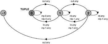
Figure 11.8: TUPLE LTS.

An example of a conditional operation on the tuple space would be:

 inp[b:Bool][t:Tuples]

The value of the local variable t is only valid when b is true. Each TUPLE process has in its alphabet the operations on one specific tuple value. The alphabet of TUPLESPACE is defined by the set TupleAlpha:

 set TupleAlpha   = {{in,out,rd,rdp[Bool],inp[Bool]}.Tuples}

A process that shares access to the tuple space must include all the actions of this set in its alphabet.

Tuple Space Implementation

Linda tuple space can be distributed over many processors connected by a network. However, for demonstration purposes we describe a simple centralized implementation that allows matching of templates only on the tag field of a tuple. The interface to our Java implementation of a tuple space is listed in Program 11.5.

Program 11.5: TupleSpace interface.

 public interface TupleSpace {   // deposits data in tuple space   public void out (String tag, Object data);   // extracts object with tag from tuple space, blocks if not available   public Object in (String tag)                     throws InterruptedException;   // reads object with tag from tuple space, blocks if not available   public Object rd (String tag)                     throws InterruptedException;   // extracts object if available, return null if not available   public Object inp (String tag);   // reads object if available, return null if not available   public Object rdp (String tag); }

We use a hash table of vectors to implement the tuple space (Program 11.6). Although the tuple space is defined to be unordered, for simplicity, we have chosen to store the tuples under a particular tag in FIFO order. New tuples are appended to the end of a vector for a tag and removed from its head. For simplicity, a naive synchronization scheme is used which wakes up all threads whenever a new tuple is added. A more efficient scheme would wake up only those threads waiting for a tuple with the same tag as the new tuple.

Program 11.6: TupleSpaceImpl class.

 class TupleSpaceImpl implements TupleSpace {   private Hashtable tuples = new Hashtable();   public synchronized void out(String tag,Object data){     Vector v = (Vector) tuples.get(tag);     if (v == null) {       v = new Vector();       tuples.put(tag,v);     }     v.addElement(data);     notifyAll();   }   private Object get(String tag, boolean remove) {     Vector v = (Vector) tuples.get(tag);     if (v == null) return null;     if (v.size() == 0) return null;     Object o = v.firstElement();     if (remove) v.removeElementAt(0);     return o;   }   public synchronized Object in (String tag)                   throws InterruptedException {     Object o;     while ((o = get(tag,true)) == null) wait();     return o;   }   public Object rd (String tag)                   throws InterruptedException {     Object o;     while ((o = get(tag,false)) == null) wait();     return o;   }   public synchronized Object inp (String tag) {     return get(tag,true);   }   public synchronized Object rdp (String tag) {     return get(tag,false);   } }

11.2.2 Supervisor – Worker Model

We model a simple Supervisor – Worker system in which the supervisor initially outputs a set of tasks to the tuple space and then collects results. Each worker repetitively gets a task and computes the result. The algorithms for the supervisor and each worker process are sketched below:

 Supervisor::   forall tasks: out(“task”,...)   forall results: in(“result”,...)   out(“stop”) Worker::   while not rdp(“stop”) do     in(“task”,...)     compute result     out(“result”,...)

To terminate the program, the supervisor outputs a tuple with the tag “stop” when it has collected all the results it requires. Workers run until they read this tuple. The set of tuple values and the maximum number of copies of each value are defined for the model as:

 const N      = 2 set   Tuples = {task,result,stop}

The supervisor outputs N tasks to the tuple space, collects N results and then outputs the “stop” tuple and terminates.

 SUPERVISOR   = TASK[1], TASK[i:1..N] =   (out.task ->      if i<N then TASK[i+1] else RESULT[1]), RESULT[i:1..N] =   (in.result ->      if i<N then RESULT[i+1] else FINISH), FINISH =   (out.stop  -> end -> STOP) + TupleAlpha.

The worker checks for the “stop” tuple before getting a task and outputting the result. The worker terminates when it reads “stop” successfully.

 WORKER =   (rdp[b:Bool].stop->     if (!b) then       (in.task -> out.result -> WORKER)     else       (end -> STOP)   )+TupleAlpha.

The LTS for both SUPERVISOR and WORKER with N=2 is depicted in Figure 11.9.

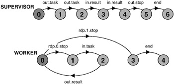
Figure 11.9: SUPERVISOR and WORKER LTS.

In the primes sieve example, we arranged that the behavior was cyclic to avoid detecting a deadlock in the case of correct termination. An alternative way of avoiding this situation is to provide a process that can still engage in actions after the end action has occurred. We use this technique here and define an ATEND process that engages in the action ended after the correct termination action end occurs.

 ATEND   = (end->ENDED), ENDED = (ended->ENDED).

A Supervisor – Worker model with two workers called redWork and blueWork, which conforms to the architecture of Figure 11.7, can now be defined by:

 ||SUPERVISOR_WORKER     = ( supervisor:SUPERVISOR       || {redWork,blueWork}:WORKER       || {supervisor,redWork,blueWork}::TUPLESPACE       || ATEND       )/{end/{supervisor,redWork,blueWork}.end}.

Analysis

Safety analysis of this model using LTSA reveals the following deadlock:

 Trace to DEADLOCK:     supervisor.out.task     supervisor.out.task     redWork.rdp.0.stop           – rdp returns false     redWork.in.task     redWork.out.result     supervisor.in.result     redWork.rdp.0.stop           – rdp returns false     redWork.in.task     redWork.out.result     supervisor.in.result     redWork.rdp.0.stop           – rdp returns false     supervisor.out.stop     blueWork.rdp.1.stop          – rdp returns true

This trace is for an execution in which the red worker computes the results for the two tasks put into tuple space by the supervisor. This is quite legitimate behavior for a real system since workers can run at different speeds and take different amounts of time to start. The deadlock occurs because the supervisor only outputs the “stop” tuple after the red worker attempts to read it. When the red worker tries to read, the “stop” tuple has not yet been put into the tuple space and, consequently, the worker does not terminate but blocks waiting for another task. Since the supervisor has finished, no more tuples will be put into the tuple space and consequently, the worker will never terminate.

This deadlock, which can be repeated for different numbers of tasks and workers, indicates that the termination scheme we have adopted is incorrect. Although the supervisor completes the computation, workers may not terminate. It relies on a worker being able to input tuples until it reads the “stop” tuple. As the model demonstrates, this may not happen. This would be a difficult error to observe in an implementation since the program would produce the correct computational result. However, after an execution, worker processes would be blocked and consequently retain execution resources such as memory and system resources such as control blocks. Only after a number of executions might the user observe a system crash due to many hung processes. Nevertheless, this technique of using a “stop” tuple appears in an example Linda program in a standard textbook on concurrent programming!

A simple way of implementing termination correctly would be to make a worker wait for either inputting a “task” tuple or reading a “stop” tuple. Unfortunately, while this is easy to model, it cannot easily be implemented since Linda does not have an equivalent to the selective receive described in Chapter 10. Instead, we adopt a scheme in which the supervisor outputs a “task” tuple with a special stop value. When a worker inputs this value, it outputs it again and then terminates. Because a worker outputs the stop task before terminating, each worker will eventually input it and terminate. This termination technique appears in algorithms published by the designers of Linda (Carriero and Gelernter, 1989b). The revised algorithms for supervisor and worker are sketched below:

 Supervisor::         forall tasks:- out(“task”,...)         forall results:- in(“result”,...)         out(“task”,stop) Worker::         while true do                 in(“task”,...)                 if value is stop then out(“task”,stop); exit                 compute result                 out(“result”,...)

The tuple definitions and models for supervisor and worker now become:

 set Tuples  = {task,task.stop,result} SUPERVISOR   = TASK[1], TASK[i:1..N] =   (out.task ->      if i<N then TASK[i+1] else RESULT[1]), RESULT[i:1..N] =   (in.result ->      if i<N then RESULT[i+1] else FINISH), FINISH =   (out.task.stop -> end -> STOP)   + TupleAlpha. WORKER =   (in.task -> out.result -> WORKER   |in.task.stop -> out.task.stop -> end ->STOP   ) + TupleAlpha.

The revised model does not deadlock and satisfies the progress property:

 progress END = {ended}

A sample trace from this model, which again has the red worker computing both tasks, is shown in Figure 11.10.

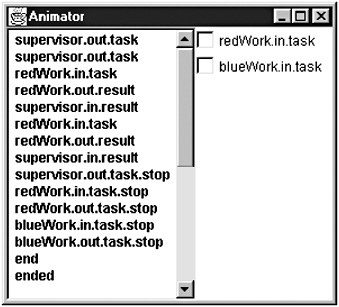
Figure 11.10: Trace of Supervisor – Worker model.

In the first section of this chapter, the primes sieve application was modeled in some detail. We then abstracted from the application to investigate the concurrent properties of the Filter Pipeline architecture. In this section, we have modeled the Supervisor – Worker architecture directly without reference to an application. We were able to discover a problem with termination and provide a general solution that can be used in any application implemented within the framework of the architecture.

11.2.3 Supervisor – Worker Implementation

To illustrate the implementation and operation of Supervisor – Worker architectures, we develop a program that computes an approximate value of the area under a curve using the rectangle method. More precisely, the program computes an approximate value for the integral:

The rectangle method involves summing the areas of small rectangles that nearly fit under the curve as shown in Figure 11.11.

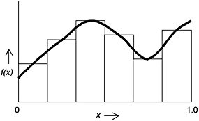
Figure 11.11: Rectangle method.

In the Supervisor – Worker implementation, the supervisor determines how many rectangles to compute and hands the task of computing the area of the rectangles to the workers. The demonstration program has four worker threads each with a different color attribute. When the supervisor inputs a result, it displays the rectangle corresponding to that result with the color of the worker. The display of a completed computation is depicted in Figure 11.12.

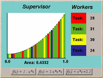
Figure 11.12: Supervisor – Worker applet.

Each worker is made to run at a different speed by performing a delay before outputting the result to the tuple space. The value of this delay is chosen at random when the worker is created. Consequently, each run behaves differently. The display of Figure 11.12 depicts a run in which some workers compute more results than others. During a run, the number of the task that each worker thread is currently computing is displayed. The last task that the worker completed is displayed at the end of a run. The class diagram for the demonstration program is shown in Figure 11.13.

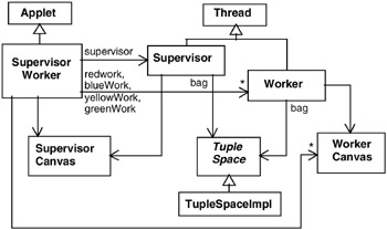
Figure 11.13: Supervisor – Worker class diagram.

The displays for the supervisor and worker threads are handled, respectively, by the classes SupervisorCanvas and WorkerCanvas. The methods provided by these classes, together with a description of what they do, are listed in Program 11.7.

Program 11.7: SupervisorCanvas, WorkerCanvas and Function classes.

 class SupervisorCanvas extends Canvas {   // display rectangle slice i with color c, add a to area field   synchronized void setSlice(               int i,double a,Color c) {...}   // reset display to clear rectangle slices and draw curve for f   synchronized void reset(Function f) {...} } class WorkerCanvas extends Panel {   // display current task number val   synchronized void setTask(int val) {...} } interface Function {   double fn(double x); } class OneMinusXsquared implements Function {   public double fn (double x) {return 1-x*x;} } class OneMinusXcubed implements Function {   public double fn (double x) {return 1-x*x*x;} } class XsquaredPlusPoint1 implements Function {   public double fn (double x) {return x*x+0.1;} }

The interface for the function f(x) together with three implementations are also included in Program 11.7.

A task that is output to the tuple space by the supervisor thread is represented by a single integer value. This value identifies the rectangle for which the worker computes the area. A result requires a more complex data structure since, for display purposes, the result includes the rectangle number and the worker color attribute in addition to the computed area of the rectangle. The definition of the Result and the Supervisor classes is listed in Program 11.8.

Program 11.8: Result and Supervisor classes.

 class Result {   int task;   Color worker;   double area;   Result(int s, double a, Color c)     {task =s; worker=c; area=a;} } class Supervisor extends Thread {   SupervisorCanvas display;   TupleSpace bag;   Integer stop = new Integer(-1);   Supervisor(SupervisorCanvas d, TupleSpace b)     { display = d; bag = b; }   public void run () {     try {       // output tasks to tuplespace       for (int i=0; i<SupervisorCanvas.Nslice; ++i)         bag.out("task",new Integer(i));       // collect results       for (int i=0; i<display.Nslice; ++i) {         Result r = (Result)bag.in("result");         display.setSlice(r.task,r.area,r.worker);       }       // output stop tuple       bag.out("task",stop);     } catch (InterruptedException e){}   } }

The supervisor thread is a direct translation from the model. It outputs the set of rectangle tasks to the tuple space and then collects the results. Stop is encoded as a “task” tuple with the value –1, which falls outside the range of rectangle identifiers. The Worker thread class is listed in Program 11.9.

Program 11.9: Worker class.

 class Worker extends Thread {   WorkerCanvas display;   Function func;   TupleSpace bag;   int processingTime = (int)(6000*Math.random());   Worker(WorkerCanvas d, TupleSpace b, Function f)     { display = d; bag = b; func = f; }   public void run () {     double deltaX = 1.0/SupervisorCanvas.Nslice;     try {       while(true){         // get new task from tuple space         Integer task = (Integer)bag.in("task");         int slice = task.intValue();         if (slice <0) {   // stop if negative             bag.out("task",task);             break;         }         display.setTask(slice);         sleep(processingTime);         double area           = deltaX*func.fn(deltaX*slice+deltaX/2);         // output result to tuple space         bag.out( "result",            new Result(slice,area,display.worker));       }     } catch (InterruptedException e){}   } }

The choice in the worker model between a task tuple to compute and a stop task is implemented as a test on the value of the task. The worker thread terminates when it receives a negative task value. The worker thread is able to compute the area given only a single integer since this integer indicates which “slice” of the range of x from 0 to 1.0 for which it is to compute the rectangle. The worker is initialized with a function object.

The structure of supervisor, worker and tuple space is constructed by the go() method of the SupervisorWorker applet class. The code is listed below:

 private void go(Function fn) {   display.reset(fn);   TupleSpace bag = new TupleSpaceImpl();   redWork = new Worker(red,bag,fn);   greenWork = new Worker(green,bag,fn);   yellowWork = new Worker(yellow,bag,fn);   blueWork = new Worker(blue,bag,fn);   supervisor = new Supervisor(display,bag);   redWork.start();   greenWork.start();   yellowWork.start();   blueWork.start();   supervisor.start(); }

where display is an instance of SupervisorCanvas and red, green, yellow and blue are instances of WorkerCanvas.

Speedup and Efficiency

The speedup of a parallel program is defined to be the time that a sequential program takes to compute a given problem divided by the time that the parallel program takes to compute the same problem on N processors. The efficiency is the speedup divided by the number of processors N. For example, if a problem takes 12 seconds to compute sequentially and 4 seconds to compute on six processors, then the speedup is 3 and the efficiency 0.5 or 50%.

Unfortunately, the demonstration Supervisor – Worker program would not exhibit any speedup if executed on a multiprocessor with a Java runtime that scheduled threads on different processors. The most obvious reason for this is that we have introduced delays in the worker threads for display purposes. However, there is a reason that provides a more general lesson.

The amount of CPU time to compute each task in the example is very small, since each task requires only a few arithmetic operations. The supervisor uses more CPU time putting the task into tuple space and retrieving the result than it would if it computed the task locally. Speedup of greater than unity is only achieved in Supervisor – Worker programs if the tasks require significantly more computation time than the time required for communication with the workers.

The advantage of the Supervisor – Worker architecture is that it is easy to develop a parallel version of an existing sequential program in which sub-problems are independent. Often the sub-problem solution code from the sequential program can be reused directly in the parallel version. In practice, the architecture has been successfully applied to computation-intensive problems such as image rendering using ray-tracing techniques.