Section 12.2. Advanced Lookups | Excel 2007[c] The Missing Manual

12.2. Advanced Lookups

VLOOKUP( ) and HLOOKUP( ) work well for linking together tables in a worksheet. They also impose a few restrictions, however, including:

The lookup column must be the first column or row in the range. That means you can't use VLOOKUP( ) to retrieve columns to the left of the lookup column, and you can't use HLOOKUP( ) to retrieve rows above the lookup row.
You must choose between horizontal and vertical lookups. You can't perform a lookup that finds cells based on a lookup column and a lookup row.

In this section, you'll learn how to skirt these restrictions with the help of other functions.

Tip: You simply can't get around certain lookup rules. The lookup functions aren't much use if you have potentially multiple matches. That means you can't use a lookup function to retrieve your top-10 selling products, for example. If you want to use this sort of logic, then you should probably opt for Excel's list feature (Chapter 14), which provides filtering capabilities.

12.2.1. MATCH( ): Finding the Position of Items in a Range

The MATCH( ) function lets you find the position of an item in a range. On its own, MATCH( ) doesn't accomplish a whole lot, but when used in conjunction with some of the functions described later in this section, you'll find it's really handy. Here are some MATCH( ) fundamentals.

To use Match( ), you simply specify the search value (either a number or text) and the range you want to search:

 MATCH(search_for, range, [match_type])

The range you use must be one-dimensional. That means you can search through the column of cells A1:A10 or the row of cells A1:E1, but you can't search the grid of cells A1:E10.

The match_type argument's optional, but highly recommended. It can take one of these three values:

. Gives you the position of the first item that matches exactly.
1 . Gives you the position of the largest value that's equal to or less than the search argument. In order for this argument to work correctly, you must perform a lookup in a range of numbers or text values that are ordered in ascending order. If you use the formula =MATCH(100, {12,23,48,101,321}, 1) , the result is 3 because the third value in the range (48) is the largest number less than 100.
1 . Gives you the position of the smallest value that's equal to or greater than the search argument. In order for this argument to work correctly, you must perform a lookup in a range of numbers or text values that are ordered in descending order. If you use the formula =MATCH("b", {"dough-nut","cracker"," banana ","apple"},1) , the result is 3 because the third value in the range (banana) is the smallest text value that falls after b in dictionary order.

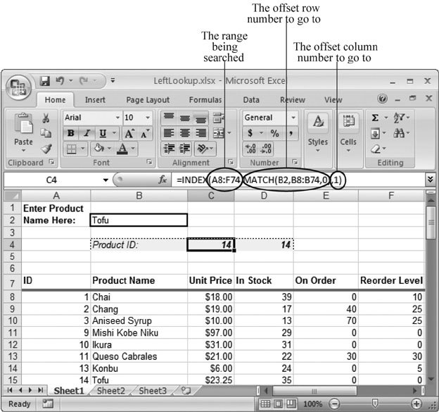
Note: You'll almost always want to use a match_type of 0. However, the MATCH( ) function uses a match_type of 1 if you omit the match_type parameter. Consider yourself warned .

If MATCH( ) finds the value you're searching for, then it gives you a number indicating its position. If you're searching the range of cells A1:A10, and the search item's in cell A3, then the MATCH( ) function returns 3 (because it's the third cell in this range). If it finds no match, MATCH( ) returns #N/A.

12.2.2. INDEX( ): Retrieving the Value from a Cell

You may have already noticed that the MATCH( ) function really does half the work of the VLOOKUP( ) and HLOOKUP( ) functions. It can find the position of the search item, but it gives you the position as an index number, instead of the actual cell content. (Index 1 is the first item in a range, 2 is the second, and so on.) The MATCH( ) function becomes useful only when you combine it with another function, like INDEX( ).

INDEX( ) is powerful not only because it can retrieve the actual cell content but also because it lets you move to any row or column you want. The next section shows you how useful that feature is. But first, here's a quick look at how INDEX( ) works.

INDEX( ) gives you a value from a range of cells, using the index number you specify:

 INDEX(range, row_number, [column_number]

Consider the following formula:

 =INDEX(A2:A10, 3)

This formula returns the content of the third cell in the range: A4. If you supply a two-dimensional range, you need to give a row and column index. Here's an example:

 =INDEX(A2:B10, 3, 2)

This formula gives you the cell in the third row and the second column, which is B4.

Note: Remember that the index numbers used by MATCH( ) and INDEX( ) are offsets, not actual cell references. In other words, if you specify a range that starts on cell E10, Excel designates E10 as index number 1, E11 as index number 2, and so on. The actual row number in the worksheet doesn't matter.

12.2.3. Performing a "Left Lookup"

On their own, MATCH( ) and INDEX( ) are just curiosities. But when you combine them, you have the ability to overcome many of the limitations inherent in VLOOKUP( ) and HLOOKUP( ).

Consider the worksheet in Figure 12-3. Here, Excel performs the lookup using column B (the product name ), and the formula retrieves information from column A (the product ID). This example's a left lookup , something that isn't possible using the VLOOKUP( ) function.

To solve this problem, you first use MATCH( ) to find the position of the product name you're looking for:

 =MATCH(B2, B8:B74, 0)

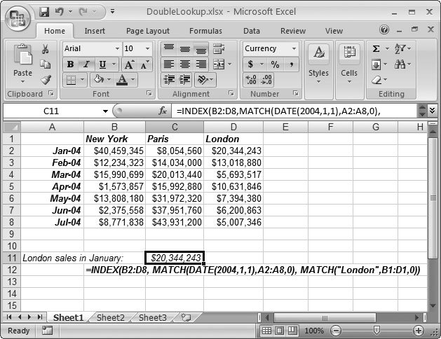
Figure 12-3. This worksheet is designed to let you search for a product by name, and then retrieve its corresponding ID information. Because the ID info is to the left of the lookup column, VLOOKUP( ) doesn't help. The solution is to combine MATCH( ) and INDEX( ), so that MATCH( ) gives you the offset row number from the Product Name column. INDEX( ) then uses that value in the ID column. Excel displays the final resultthe product IDin cell C4, which contains the formula that's doing all the work. In essence, this formula breaks the problem down into two questions: "How far down is this product name?" and "What product ID is just as far down?" MATCH( ) answers the first question, while INDEX( ) answers the second.

This formula gives you a value of 8 because the searched for value (Tofu) is located in the eighth row of the cell range you're searching. Next, you can use the value from the MATCH( ) function to retrieve the cell content by employing the INDEX( ) function. The trick is that the INDEX( ) function uses a range that covers all the rows and columns in the table of data:

 =INDEX(A8:F74, match_result, 1)

Here's how you'd combine these functions into a single formula:

 =INDEX(A8:F74, MATCH(B2,B8:B74,0), 1)

Tip: Remember, the INDEX( ) function lets you perform a lookup in a column or a row.

12.2.4. Performing a Double Lookup

Another shortcoming with the VLOOKUP( ) and HLOOKUP( ) functions is that you can't use them simultaneously . These functions don't help if you want to write a formula that finds a cell at the intersection of a specific column and row heading. Imagine you want to write a formula to find the number of sales recorded in January 2004 at the London location, in the spreadsheet shown in Figure 12-4. You can solve this problem with the INDEX( ) function, which is much more flexible than either the VLOOKUP( ) or the HLOOKUP( ) function.

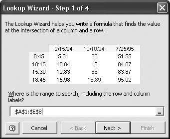
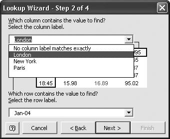
Figure 12-4. The formula in cell C11 performs a double lookup by using MATCH( ) twice to get the offsets, and INDEX( ) once to retrieve the value. This method works because the INDEX( ) function accepts both a row and a column offset.

Note: With just a tad more work, you can write a formula that lets readers of your spreadsheet indicate which city and which month they're interested in seeing sales figures for. Those steps are covered in the next section.

Because you need to look up the rows and columns, you'll need to use the MATCH( ) function twice.

First, you'd use the MATCH( ) function to find the row that has the January sales figures:

 =MATCH(DATE(2004,1,1), A2:A8, 0)

Note: Remember that the DATE( ) function, as explained in Section 11.4.2, creates a date without your needing to know its underlying serial number.

Next, you'd use MATCH( ) to find the column with the sales figures for the London office:

 =MATCH("London", B1:D1, 0)

With these two pieces of information, you can build an INDEX( ) function that searches the whole range for the appropriate sales figure:

 =INDEX(B2:D8, MATCH(DATE(2004,1,1),A2:A8,0), MATCH("London",B1:D1,0))

In this example, the search values (the date and the store location) are hard-coded in the formula, but you can just as easily retrieve this information from another cell.

12.2.5. The Lookup Wizard

If you're becoming a little frazzled from considering all the different types of lookup functions, you may be glad to learn that Excel includes a tool that builds lookup functions for you automatically . It's called the Lookup wizard.

Here's how you'd use the Lookup wizard to build the sales lookup formula used in the previous example.

If this is the first time you're using the Lookup wizard, you need to switch it on. Choose Office button Excel Options .

If this isn't the first time you're using the Lookup wizard, skip to step 5.
In the Excel Options window, pick the Add-Ins category .

This category shows a list of all the currently active add-ins, and those that are installed but not active. (Add-ins are tiny software programs that integrate with Excel to provide additional features.) Microsoft provides some add-ins, but other companies develop and sell many more.
In the Manage box at the bottom of the window, choose Excel Add-Ins, and then click Go .

The Add-Ins window appears, which lets you switch your add-ins on or off.
Place a checkmark next to Lookup wizard, and then click OK .

You may need to insert the Office (or Excel) DVD you got when you originally bought Excel in order to install the Lookup wizard add-in. Once you have the add-in installed and switched on, you'll find an additional entry in the ribbon's Formulas tab.
Launch the Lookup wizard by selecting Formulas Solutions Lookup .

The Lookup wizard dialog box opens (Figure 12-5).
Select the range of cells where you'd like to perform the lookup, and then click Next .

In the sales example, this is the range A1:D8. Make the selection by dragging across the cell range on the worksheet.

Figure 12-5. You can get help writing lookup formulas with Excel's Lookup wizard, which walks you through a series of questions. First choose the range you're searching.
Specify both the row and column that form the intersection of the cell you're looking to identify .

You can make your choices from the wizard's two drop-down lists (see Figure 12-6).

Figure 12-6. Choose the column you want from the top drop-down list and choose the row from the bottom list. In the sales example, the column is London and the row is Jan-04.

Choose whether to display just the formula you've created or the formula plus the two lookup parameters (Figure 12-7). Once you've made your choice, click Next to continue .

Choosing just the formula is only moderately helpful, because the wizard creates a formula that's hard-coded with the two lookup parameters. Translation: The formula works, but it gives you only the value of the cell that lies at the intersection you've identified.

On the other hand, if you choose to display the formula plus the two lookup parameters, things get interesting. In this case, you can modify your lookup parameters at any time to identify different cells within your table. You'll appreciate that kind of flexibility if you want your spreadsheet readers to specify the city and date they'd like to see.

Once again, in the sales example, the Lookup wizard would add two extra cells (as explained in the next step)one with the text London and one with the date January 1, 2003. The lookup formula references these cells, so if you change the word London to Paris, the lookup result changes automatically.

Figure 12-7. One nice feature of the Lookup wizard is that it can insert the lookup arguments into separate cells. This way, readers can search your spreadsheet for different data just by editing these cells.

Finally, choose where you want to put the formula (by clicking on the worksheet), and click Finish .

If you opted to insert a formula plus the lookup parameters, you go through two additional steps to fill the cells with the lookup criteria.

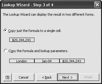
Here's what the completed formula could look like, if you chose to let the Lookup wizard also use lookup parameters:

 =INDEX($A:$D, MATCH(F5,$A:$A,), MATCH(F4,$A:$D,))

As you can see, this formula uses the MATCH( ) and INDEX( ) function, just as in the previous section. However, it doesn't supply the recommended match_type parameter. It's a good idea to edit the formula by setting the match_type to 0, in order to ensure that any data your readers type into the spreadsheet matches your lookup parameters exactly:

 =INDEX($A:$D, MATCH(F5,$A:$A,0), MATCH(F4,$A:$D,0))

Excel's version of the formula also uses absolute references (Section 8.3.1), which ensures that the cell reference doesn't change if you copy the formula to another area on the worksheet.

Note: The Lookup wizard works wonders if your data is set out in a typical table with column and row headings, but it's less flexible when your data's organized in an unconventional way, or if you need to perform a lookup in two different areas on the worksheet. In the latter cases, the INDEX( ) and MATCH( ) functions are still up to the task, although you'll need to exert a little more brainpower creating a formula that uses them.

12.2.6. OFFSET( ): Moving Cell References to a New Location

Not surprisingly, Excel gives you another way to solve lookup problems. The OFFSET( ) function lets you take a cell reference and move it to a new location. If you take the cell reference A1, and use OFFSET( ) to move it down two rows, then Excel would refer to it as cell A3.

For the most part, everything you can accomplish with the OFFSET( ) function you can also achieve by combining INDEX( ) and MATCH( ). It's really a matter of preference. Some Excel gurus prefer to use INDEX( ) and MATCH( ), while others find that OFFSET( ) makes for clearer formulas. Once you've finished this section, you'll be able to make your own choice.

The OFFSET( ) function requires three arguments: the cell reference you want to move, the number of rows you want to move, and the number of columns you want to move:

 OFFSET(reference, rows_to_offset, cols_to_offset, [height], [width])

The following formula moves the reference A1 to A3, and then returns whatever content's in that cell:

 =OFFSET(A1, 2, 0)

To move a row upwards or to a column that's to the left, specify a negative number for the rows_to_offset or cols_to_offset parameter, respectively. You can also use the height and width parameters to expand the cells your reference covers, converting it from a single-cell reference into a full-fledged range. Here's one example:

 =SUM(OFFSET(D2, 0, 0, 7, 1))

This formula uses OFFSET( ) to expand a reference (D2) to a range containing seven cells (D2:D8). The original cell serves as the "anchor point" that becomes a corner in the range. Then Excel passes on that range to the SUM( ) function. The end result is equivalent to this formula:

 =SUM(D2:D8)

Now that you understand OFFSET( ), you can use it in place of the INDEX( ) function in most situations. You just need to start at the top-left corner of your table, and use the OFFSET( ) function to get to the cell you want.

Consider the formula in Figure 12-3, which performs a left lookup on the product list:

 =INDEX(A8:F74, MATCH(B2,B8:B74,0), 1)

You can easily rewrite this using the OFFSET( ) function, as shown here. Cell A8, at the top-left corner of the table, is the starting point:

 =OFFSET(A8, MATCH(B2,B8:B74,0)-1, 0)

Like those in the INDEX( ) section (Section 12.2.3), this formula still lets you search through the entire table of data to find the Product Name (using the Product ID value you typed in). In fact, there's really no meaningful difference between the two functions. In most cases, you can use OFFSET( ) or INDEX( ) interchangeably. One exception is that only the OFFSET( ) function has the ability to convert a single-cell reference into a range.

12.2.7. Other Reference and Lookup Functions

MATCH(), INDEX( ), and OFFSET( ) are definitely the three most useful reference and lookup functions. However, Excel also provides a few more similar functions that occasionally come in handy. Table 12-1 gives you a quick tour.

Table 12-1. Miscellaneous Reference and Lookup Functions

Function	Syntax	Description
AREAS( )	AREAS(reference)	Returns the number of areas in a reference. An area is a single cell or a range of contiguous cell. If you have more than one area, all the areas need to be enclosed within double parentheses. For example, =AREAS(A1) returns a value of 1; =AREAS((A1, B3:D5, E8)) returns a value of 3.
COLUMN( )	COLUMN(reference)	Returns the column number for a reference. =COLUMN(B3) returns the number 2, which represents column B. If you leave out the reference, then you get the column number of the current cell (the cell that holds your formula).
COLUMNS( )	COLUMNS(range)	Counts the number of columns in a range.
ROW( )	ROW(reference)	Returns the row number for a reference. =ROW(B3) returns the number 3. If you leave out the reference, then you get the row number of the current cell (the cell that holds your formula).
ROWS( )	ROWS(range)	Counts the number of rows in a range.
CHOOSE( )	CHOOSE(index_num, value1, value2, )	Returns a value from a list depending on the index number. For example, =CHOOSE(1, A1, A2, B1) returns the content in cell A1 because that's the first position in the list of values that follows .
LOOKUP( )	LOOKUP(search_for, lookup_range, result_ range)	LOOKUP( ) is a slimmed-down version of HLOOKUP( ) and VLOOKUP( ). It searches for a value in one range, and returns the value in the same index position in the second range. Unfortunately, you've no way to enforce strict matching, which reduces the usefulness of this function.

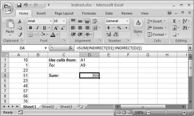
12.2.8. INDIRECT( ) and ADDRESS( ): Working with Cell References Stored As Text

INDIRECT( ) and ADDRESS( ) are two of Excel's strangest reference functions. They let you work with cell references stored as text.

The INDIRECT( ) function retrieves the content from any cell you specify. The twist is that you specify the cell using literal text (a string) to describe the location of the cell. So, where normally you would add two cells this way:

 =A1+A2

if you were to use INDIRECT( ) to refer to cell A1, you'd write the formula this way:

 =INDIRECT("A1")+A2

Note the quotation marks around the cell name; they indicate that A1 is just a piece of text, not a cell reference. The INDIRECT( ) function examines this text and gives you the corresponding cell reference.

The obvious question is why would anyone bother to specify cell references as ordinary text? The most common reason is because you want to create a formula that's extremely flexible. So, for example, instead of hard-coding your cell references (as in =A1+A2), you may want your formula to read another cell to find out which cell reference it should use. The end result is that the person reading the spreadsheet can change a cell reference used in a calculation, without needing to edit a complex formula by hand. Figure 12-8 shows a worksheet that demonstrates this trick. It lets the person using the spreadsheet choose the numbers to add, without forcing him to write a SUM( ) function by hand.

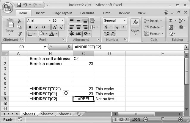
Figure 12-8. This worksheet shows the quirky INDIRECT( ) function at work. Here, a dynamic SUM( ) formula is used to add a range of cells. The SUM( ) formula uses the INDIRECT( ) function to read the cell references stored in cells D1 and D2. It then uses these to create the range of cells that are added together.

Here's an example of this technique:

 =INDIRECT(A1)+INDIRECT(A2)

This formula does not add the content of cells A1 and A2. Instead, it looks in the cells A1 and A2 to determine which two cells it should add together. If the cell A1 contains the text "B2" and the cell A2 contains the text "D8", the formula becomes the following:

 =INDIRECT("B2")+INDIRECT("D8")

which is the same as:

 =B2+D8

This formula assumes that there are two cell references, entered as text, in cells A1 and A2. If there's something else in these cells, the INDIRECT( ) function doesn't work. If cell A1 contains a number, for instance, the formula INDIRECT(A1) returns the error code #REF! (which is Excel shorthand for, "I expected a cell reference, but all you gave me was a lousy number"). Figure 12-9 shows what you canand can'tdo with the INDIRECT( ) function.

Figure 12-9. This worksheet shows three attempts at using INDIRECT( ). In C7 (whose formula's written out in B7), the cell reference (C2) is a hard coded piece of text. The formula displays the value contained in cell C2. C8 has an extra layer of redirection. The formula grabs the content in C1, which is the piece of text "C2," and then supplies that to the INDIRECT( ) function. The INDIRECT( ) function then displays the content from cell C2, as in the previous example. The final =INDIRECT("C2") formula grabs the content from C2, which isn't a cell reference (it's the number 23). As a result, the INDIRECT( ) function accomplishes nothing.

The ADDRESS( ) function performs a similarly strange operation, but in reverse. You supply ADDRESS( ) with row and column index numbers, and Excel gives you a piece of text that contains the cell reference. The following formula returns $B$1:

 =ADDRESS(1, 2)

Remember, all the ADDRESS( ) function does is return a cell reference as a string. This piece of text isn't too useful; all you can really do with it is display it in a cellor, if you're really warped , pass it to the INDIRECT( ) function to convert it back to a real cell reference.

Consider the example shown in Figure 12-4, which uses a lookup function to find the sales in a particular city on a particular month. The formula looked like this:

 =INDEX(B2:D8, MATCH(DATE(2004,1,1),A2:A8,0), MATCH("London",B1:D1,0))

Instead of displaying the actual sales figures, you could use the ADDRESS( ) function to display the cell reference for the spreadsheet reader to see, like so:

 =ADDRESS(MATCH(DATE(2004,1,1),A2:A8,0), MATCH("London",B1:D1,0))

This formula displays the text $C$4. If you want to get craftier, then you could add some additional text by modifying the formula like this:

 ="The number you are looking for is in cell " & ADDRESS(MATCH(DATE(2004,1,1),A2:A8,0), MATCH("London",B1:D1,0))

This formula displays the text The number you are looking for is in cell $C$4 . Clearly, you won't use a formula like this often, but it does raise some interesting possibilities.

If you don't want the ADDRESS( ) function to return a string with an absolute reference (Section 8.3.1), then you can supply a third parameter, called abs_number . It takes one of the following values:

1 Returns an absolute address, as in $B$1.
2 Fixes the row number, as in B$1.
3 Fixes the column, as in $B1.
4 Returns a relative reference, as in B1.

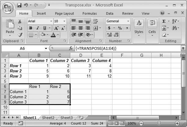
12.2.9. TRANSPOSE( ): Changing Rows into Columns and Vice Versa

TRANSPOSE( ) is an interesting function that you can use to change the structure of a table of data. Using TRANSPOSE( ), you can invert the data so that all the rows become columns, and the columns become rows (Figure 12-10). In that respect, it works the same as the Transpose option in the Paste Special dialog box, as described in Figure 3-8 in Section 3.2.4. The Paste Special approach, however, creates a distinct copy of the data. The TRANSPOSE( ) function, on the other hand, creates a linked table that's bound to the original data, which means that if you change the original table, the transposed table also changes. The TRANSPOSE( ) function is, therefore, ideal for showing more than one representation of the same data.

Figure 12-10. In this worksheet, the TRANSPOSE( ) function has inverted most of the data in a table, turning columns into rows and rows into columns.

The best way to get started with the TRANSPOSE( ) function is to try a simple example. Just follow these steps:

Find a table of cells you want to transpose. Make a note of its size in rows and columns .

To determine the size of the transposed table, simply switch the number of rows and columns. That means a table made up of three rows and four columns becomes a table made up of four rows and three columns.
Move to the area where you want to insert the transposed cells, and select the appropriately sized area .

If you want to transpose a table with three rows and two columns, then you need to select a grid of cells that's two rows high and three columns wide. You need to select all the cells before you begin because you'll be creating an array formula (Section 8.3). (You need an array formula because the TRANSPOSE( ) function returns a whole table's worth of results.)
Press the equal sign (=) and begin typing the TRANSPOSE( ) formula .

The TRANPOSE( ) formula requires one argument, which is the range of cells you want to transpose. Here's an example: =TRANSPOSE(A1:E4) . Don't press Enter yet.
Commit the function by pressing Ctrl+Shift+Enter .

This step inserts the formula into all the selected cells as an array formula.