Section 20.3. Solver | Excel 2007[c] The Missing Manual

20.3. Solver

Goal seeking works well for simple problems. But it does have a few limitations:

Excel doesn't recognize what you may think of as common-sense limits in your data . In the earlier student grade example, if you were looking to figure out the assignment grade required to obtain a final grade of 100, Excel would tell you you'd need a score of 113even though a grade over 100 percent clearly isn't possible.
Excel adjusts only one cell . There's no way to ask the goal-seeking tool, for instance, to predict the minimum grade combination you'd need on the two tests to get a particular final grade.

Solver is an Excel feature that goes several steps further than goal seeking. It uses the same basic trial-and-error approach (known to scientific types as an iterative approach), but it's dramatically more intelligent than goal seeking. In fact, it needs to be much more intelligent because it tackles much more complicated problems, including scenarios that have multiple changing cells , additional rules, and subtle relationships. Solver can (with a fair bit of work) suggest an optimal investment portfolio based on a desired rate of return and risk threshold. Incidentally, Solver is an add-in that you have to turn on the first time you use it; Section 20.3.2 tells you how.

Note: Although it comes as part of the Excel package, the Solver add-in isn't a Microsoft product. Instead, it's provided by a company called Frontline Systems, which sells more enhanced versions of the Solver tool. To find out about these or to look through a number of interesting (and complicated) sample worksheets that demonstrate Solver in action, go to www.solver.com.

20.3.1. Understanding Solver

Every problem that Solver is capable of solving contains the same basic ingredients. Altogether, these ingredients make up a Solver model . They include:

Target cell . The target cell is the value you want to optimize. As with goal seeking, you work with only one target cell at a time. However, you don't have to set a specific numeric goal for the target cell. Instead, you can ask Solver to just make the target value as large or small as possible (without violating the other rules of the model). The function in the target cell is the objective function .
Changing cells . These cells contain the values (also known as decision variables ) that Solver modifies in order to reach the target you want. Unlike goal seeking, you can designate multiple changing cells. When you do, Solver tries to adjust them all at once and gauge the most significant factors. With multiple changing cells, there's a definite possibility for multiple solutions (there's more than one combination of grades that can lead to a final grade of 80 percent). However, Solver stops when it finds the first matching solution.
Unchanging cells . Unchanging cells can contain values that affect the calculation that's used in the target cell. However, Solver never changes these cells.

Tip: Sometimes, it's useful to combine Solver with Excel scenarios. You may want to create multiple scenarios, each of which has different values for the unchanging cells.
Constraints . Constraints are rules that you use to restrict possible solutions. Usually, you apply constraints to changing cell values. People often add constraints that set a maximum and minimum allowed value for each changing cell. You can also use constraints to restrict the target value. You could ask Solver to find the maximum value for the target cell, but add a constraint indicating that this value can't fall in a certain range.

Note: Solver doesn't enforce constraints absolutely . Instead, it permits a certain tolerance range , depending on the configuration options that you've enacted. If you specify that a certain changing cell needs to be less than or equal to 100, Solver allows a value of 100.0000001, because it falls (just barely ) in the standard tolerance range of 0.0000001. You'll learn how to adjust the tolerance setting later in this chapter.

You can probably already see that the service provided by Solver is similar to goal seeking, but with a few significant improvements. In the next section, you'll learn how to create a Solver model.

POWER USERS' CLINIC Store the Solver Results in a Scenario

Instead of applying the values that Solver calculates, you can store them so you can refer to them later. Solver helps you out with a nifty feature that stores Solver results in a new scenario.

To use this feature, just click the Save Scenario button in the Solver Results dialog box after the Solver calculation is finished. Enter the name for the scenario you want to create, and then click OK. Excel creates the scenario and stores the value of each changing cell. To apply the scenario values later on, select Data Data Tools What-If Analysis Scenario Manager, find the scenario in the list, and then click Show.

20.3.2. Defining a Problem in Solver

To learn how Solver works, take another look at the student grade example shown in Figure 20-7. This time, consider what happens when you add a new student named Katharine Susan. This student missed the first test and, as a result, received a score of 0 on it. She wants to know what grades in the second test and assignment she needs to guarantee her a final grade of 70. Excel's goal seeking tool can't tackle this problem. Not only is it unable to change two cells at once, but it doesn't heed any upper limits, so it cheerily recommends scores greater than 100 percent. Instead, you need Solver.

To create a Solver model for this problem, follow these steps:

If this is the first time you're using Solver, you need to switch it on. Choose Office button Excel Options .

If this isn't the first time you're using Solver, skip to step 5.
In the Excel Options window, pick the Add-Ins category .

This shows a list of all your currently active add-ins, and those that are installed but not active.
In the Manage box at the bottom of the window, choose Excel Add-Ins, and then click Go .

The Add-Ins window appears, which lets you switch your add-ins on or off.
Turn on the checkbox next to the Solver Add-in, and then click OK .

You may need to insert the Office (or Excel) CD you got when you originally bought Excel in order to install the Solver add-in. Once you have the add-in installed and switched on, you'll find an additional entry in the Data tab of the ribbon.
Launch Solver by choosing Data Analysis Solver .

The Solver Parameters dialog box appears.

In the Set Target Cell text box, enter the cell you want Solver to optimize .

In the student grade example, this is cell E10, which contains Katharine Susan's final grade (see Figure 20-12).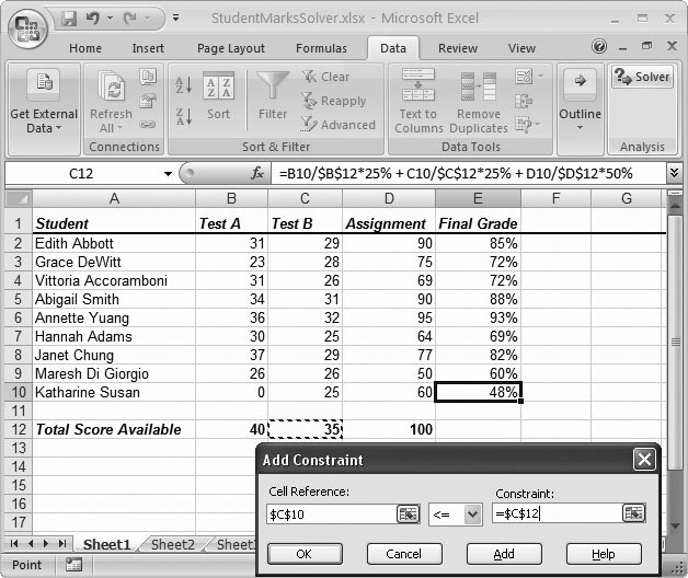

Figure 20-12. The Solver tool helps calculate the values needed in C10 and D10 to boost E10 to 70 percent. The constraint ensures the "Test B" grade isn't increased above the maximum grade available (shown in C12).

Choose the type of optimization you want by selecting one of the three Equal To options. If you choose to match a set value, enter it in the "Value of" text box .

In the student grade example, Katharine is trying to scrape past with a 70 percent grade, so the target is 0.70.
In the By Changing Cells text box, enter the cell references that Excel should modify to achieve the target .

You can enter these cell references manually (separating each reference with a comma), or you can click your worksheet to select the appropriate cells. In the student grade example, the changing cells are C10 and D10, which represent the two grades that are still up for grabs.

Now, you need to indicate the restrictions that Solver follows when it calculates its solution.
If you don't need any constraints, skip to step 12. Otherwise, click the Add button to add a constraint .

The Add Constraint dialog box appears (as shown in Figure 20-12). In the student grade example, you can use constraints to prevent scores that are above the maximum possible grade (or less than 0).
Every constraint consists of a cell reference, an operator that's used to test the cell reference, and a constraint that the cell needs to match. Enter this information, and then click OK to add the constraint .

A basic constraint compares a cell to a fixed value or another cell. You can perform an equal to comparison (=), greater than or equal to comparison (>=), or a less than or equal to comparison (<=). Figure 20-12 shows one of the constraints used in the student grade example. This constraint uses the less than or equal to (<=) operator to ensure that cell C10 (one of the changing values) doesn't exceed C12. It's not necessary to set a minimum value in this case because Solver can't solve the problem by lowering the grades.

There are also two special types of constraint operators, which show up in the list as the word int and bin . If you apply an int constraint to a cell, Solver allows that cell to contain only whole integer values (with no digits on the right side of the decimal). If you apply a bin constraint, Solver permits only binary values. In both of these cases, all you need to specify is the cell reference and the operator. You don't need to fill in the third part (the Constraint box) because it doesn't apply.

If you have another constraint to add, return to step 10. Otherwise, continue with the next step .

Figure 20-13 shows the completed Solver model.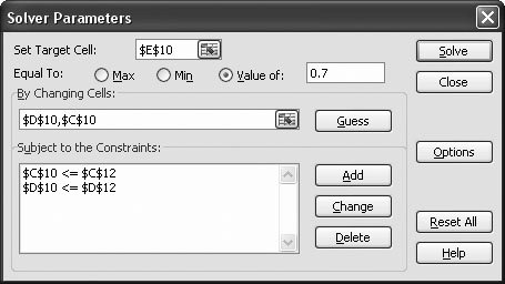

Figure 20-13. This completed Solver Parameters dialog box is ready to find out how Katharine Susan can eke out a final grade of 70. It allows for two changing cells (the test and assignment grades in cells D10 and C10), and it sets constraints to prevent solutions that don't correspond to real-world possibilities.

Click Solve to put Solver to work .

When you click Solve, the Solver Parameters dialog box disappears, and the status bar indicates the number of trial solutions in progress. You can interrupt the process at any time by pressing the Esc key. If you do, the Show Trial Solution dialog box appears, which lets you abandon your attempt altogether by clicking Stop, or resume the trial process by clicking Continue.

When Solver finishes its work, it shows the Solver Results dialog box, which indicates whether it found a solution, and what that solution is. The Solver Results dialog box also provides an option for generating a report, which you'll learn about a little later in this chapter.
Click Keep Solver Solution to retain the changed values .

To undo Solver's work and go back to the previous version, click Restore Original Values.
If you wish, in the Reports list box, choose a Solver report .

Solver gives you the option to create special reports that indicate how it calculated the answer.

The reports include Answer, Sensitivity, and Limits. Each report opens in a separate worksheet when you click OK. Most people won't find these reports very interesting at all because they contain a bare minimum of data, and what they do include are dry statistical calculations. The Solver reports aren't nearly as useful as the scenario summaries described earlier.
Finally, click OK to return to your worksheet .

Figure 20-14 shows the solution that Solver found for Katharine Susan.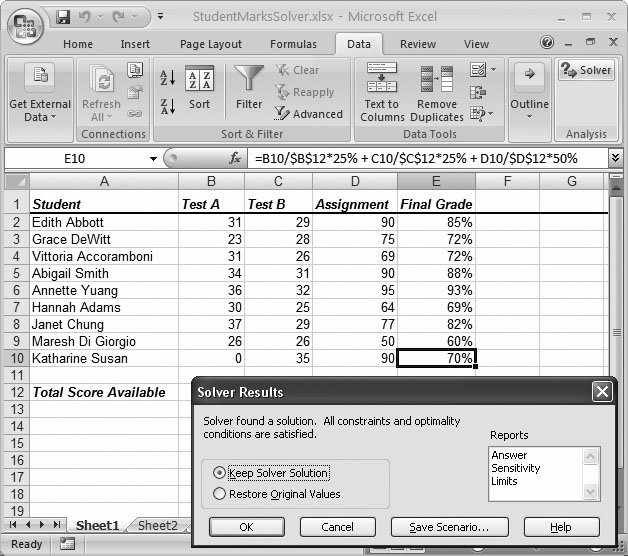

Figure 20-14. There's hope for Katharineprovided she does well on the second test and the assignment. Solver identifies a solution by increasing the test score to its maximum (35 points, which translates to 100 percent), and then by incrementing the assignment grade to 90 (out of a possible 100).

POWER USERS' CLINIC
Solver Examples

With a little imagination , you can create Solver models for a variety of scenarios. People often use Solver to find the best ways to distribute work across multiple manufacturing centers (each of which has its own operating costs and maximum production level). Or you could use Solver to plan investments, using constraints to ensure that your assets are properly distributed across different industries or geographic locations. You can learn a lot about how Solver works by looking at some example worksheets that deal with these problems.

Excel provides a workbook called solvsamp.xls that includes several examples on separate worksheets. (You can find this file in a folder like C:\Program Files\Microsoft Office\Office12\Samples . If you have trouble locating it, try using the Windows Search feature by clicking the Start button and then choosing Search.) Each worksheet has sample calculations and detailed information for using Solver, along with color -coded cells that show the target cells, changing cells, and constraints.

You can find an even more extensive collection of examples at the Solver Web site (www.solver.com/solutions.htm). There, you'll find links for several different categories, each one with several downloadable workbooks that use the same format as solvsamp.xls.

20.3.3. Advanced Solver Solutions

The student grade example shows only a hint of Solver's true analytical muscle. To see Solver tackle a more interesting problem, you can add additional constraints. You can tell Solver to make sure that the assignment grade is always higher than the test score, or that both the assignment and the test end up having equal percentage values. Figure 20-15 shows the latter example.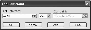

Figure 20-15. This constraint calculates the percentage on the assignment (D10/D12), and multiplies it by the total available test score (C12). The constraint forces a solution in which Katharine has an equal percentage grade on the test and on the assignment. The solution is 33 out of 35 for the test and 93 out of 100 for the assignment, both of which equal 93 percent.

Note: Solver can't optimize more than one value at once. You can't tell Solver to calculate the lowest possible grade on test B that can, in combination with the assignment score, still result in a final grade of 80. However, you can approximate many cases like this with a crafty use of constraints.

Of course, not all problems have a solution. If you repeat the same problem but try to end up with a final grade of 90 for Katharine, you'll find that it's just not possible. Solver increases both changing cells to their maximum allowed values, and then shows the Solver Results dialog box with a message informing you that there's no feasible solution.

Note: As intelligent as Solver is, it can't find all solutions, especially in complex mathematical equations that involve exponents or logarithms. If you're trying to perform some high- powered number crunching for a mathematical dissertation, you're much better off with a dedicated mathematical tool like MATLAB (www.mathworks.com/products/matlab).

20.3.4. Saving Solver Models

Each time you use Solver, Excel keeps track of the settings you've just used. And each time you save your workbook, it also saves the most recent Solver settings. However, in some cases you may want to keep track of more than one set of Solver settings. This situation could occur if you're trying to optimize the same data in different ways, or if you're using Solver to optimize data in different parts of the same worksheet or different worksheets in the same workbook. In either case, you need to explicitly save the Solver target value, changing cells, and constraints if you want to use them later.

Solver lets you save all of this information and load it later. The only catch is that you need to save it in a small block of cells in one of your worksheets. The actual number of cells you need depends on the Solver model you've created. Excel uses one cell to store information about the target value and the target cell, another cell to store the list of changing cells, and one additional cell for each constraint. The cells are stacked on top of each other.

To save a Solver model, follow these steps:

If you haven't already started Solver, choose Data Analysis Solver .

The Solver Parameters dialog box appears.
Click the Options button in the Solver Parameters dialog box .

The Solver Options dialog box appears.
Click the Save Model button in the Solver Options dialog box .

The Save Model dialog box appears.
Click inside the Select Model Area text box. Then, click the worksheet where you want to place the first cell .

Make sure that there are enough empty cells underneath the cell you select so that the Solver information doesn't overwrite any worksheet data.
Click OK .

Solver writes the information from the current model to your worksheet and returns you to the Solver Options dialog box.
Click OK or Cancel to return to the Solver Parameters dialog box .

Figure 20-16 shows what stored Solver data looks like. The cell values that you see (like TRUE and FALSE) don't have any real meaning. The real information is in the formulas inside these cells. Solver simply uses these formulas as a convenient way to store the required information in a recognizable format. The formulas don't actually calculate anything. The cell that contains the information about the target cell and target value contains the meaningless formula =$E$10=0.7.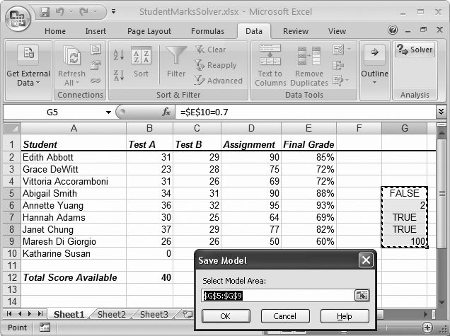

Figure 20-16. Solver uses the cells G5 to G9 to store the current scenario information.

To restore a Solver model that you saved earlier, follow these steps:

If you haven't already started Solver, choose Data Analysis Solver .

The Solver Parameters dialog box appears.
Click the Options button in the Solver Parameters dialog box .

The Solver Options dialog box appears.
Click the Load Model button in the Solver Options dialog box .

The Load Model dialog box appears.
Click inside the Select Model Area text box. Then, click the worksheet and select the cells with the Solver data .

Make sure you select all the cells. It's not enough to simply select the first cell in the list.
Click OK .

Solver reads the information from your worksheet and configures the current Solver scenario accordingly .
Click OK or Cancel to return to the Solver Parameters dialog box .

20.3.5. Configuring Solver

The standard options that Solver uses are adequate for most situations. However, if you'd like to take a closer look at how Solver works, and you want to tinker with some of Solver's advanced settings, you can configure them from the Solver Options dialog box, shown in Figure 20-17.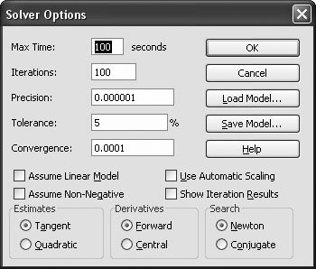

Figure 20-17. The Solver Options dialog box helps you tweak some options that control how Solver attacks a problem. Most of these enhancements are best left in the hands of experienced mathematicians (and even then, they may not improve Solver's rate of success or its performance). The most important settings are those at the top of the dialog box, which govern how long Solver can work and how exacting it must be.

To show the Solver Options dialog box, click the Options button from the main Solver Parameters dialog box (where you define your scenario). The Solver Options dialog box shows a slew of options, all of which you can change. To make your changes permanent, click OK. To return to the original settings that Solver started with, click the Reset All button in the Solver Parameters dialog box.

The most useful Solver options include:

Max Time . You can use this setting to limit the time Solver takes to a specific maximum number of seconds. You can enter a value as high as 32,767, but Solver rarely reaches the standard limit of 100 seconds in typical small problems.
Iterations . You can use this setting to limit how many trial-and-error calculations Solver makes. Once again, the number can be as high as 32,767. The only reason you would change the Max Time or Iterations setting is if Solver can't find a valid solution (in which case you may want to increase these limits), or if Solver takes an exceedingly long time without any success (in which case you may want to decrease them).
Precision . This setting indicates how exact a constraint rule needs to be. The smaller this number is (the more zeroes after the decimal place), the greater the precision, and the more exacting Solver is in trying to meet your constraints.
Tolerance . Tolerance plays a similar role to precision, but it comes into play only when you use int constraints. These constraints force one or more changing cells to be integers, in which case it's usually more difficult to get to your exact target value. To compensate, Solver is more generous in the solutions that it acceptsin fact, it accepts any solution that falls within the tolerance range of the target.
Convergence . Convergence applies to certain types of mathematical problems known as nonlinear problems . With this type of problem, Solver has a hard time telling whether its trial-and-error guesses are approaching the best solution. Each time Solver perform a new attempt, it compares its new guess to the last guess. If five guesses pass and the change is always less than the convergence value, Excel decides that it has settled on the closest solution it can find, and returns an answer. If you make the convergence smaller, Solver takes more time trying to refine its solution, and it may deliver a slightly more precise answer.
Show Iteration Results . If you turn this checkbox on, Solver pauses to show the results of each guess it makes in its trial-and-error process. This choice slows down the process tremendously, but it also gives you some interesting insight into how Solver makes its guesses.