4.2. Formatting Cell Appearance Formatting cell values is important since it helps maintain consistency among your numbers. But to really make your spreadsheet readable, you're probably going to want to enlist some of Excel's tools for controlling things like alignment, color, and borders and shading. Figure 4-6. Special number formats are ideal for formatting sequences of digits into a common pattern. For example, if you choose Phone Number in the Type list, Excel converts the sequence of digits 5551234567 into the proper phone-number style(555) 123-4567with no extra work required on your part. 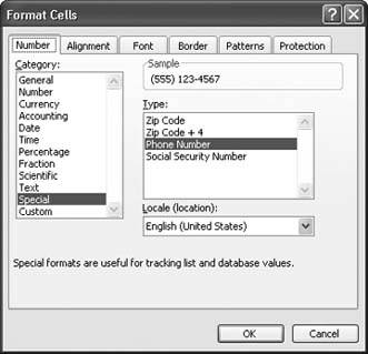
To format the appearance of a cell, first select the single cell or group of cells that you want to work with, and then choose Format  Cells from the menu, or just right-click the selection and choose Format Cells. The Format Cells dialog box that appears (Figure 4-7, top) is the place where you adjust your settings. Cells from the menu, or just right-click the selection and choose Format Cells. The Format Cells dialog box that appears (Figure 4-7, top) is the place where you adjust your settings.
Note: Even a small amount of formatting can make a worksheet easier to interpret by drawing the viewer's eye to important information. Of course, as with formatting a Word document or designing a Web page, a little goes a long way. Don't feel the need to bury your worksheet in exotic colors and styles just because you can.
4.2.1. Alignment and Orientation As you saw in the previous chapter, Excel automatically aligns cells according to the type of information you've typed in. But what if this alignment isn't what you want? Fortunately, the Alignment tab in the Format Cells dialog box (Figure 4-7, top) lets you easily change alignment as well as control some other interesting settings, like the ability to rotate text. Excel lets you control the position of content between a cell's left and right borders with the following choices, some of which are shown in Figure 4-7, bottom: General. General is the standard type of alignment; it aligns cells to the right if they hold numbers or dates and to the left if they hold text. General alignment is the type you learned about in Chapter 2. Left (Indent). Left indicates that Excel should always line up content with the left edge of the cell. You can also choose an indent value to add some extra space between the content and the left border. Center. Center indicates that Excel should always center content between the left and right edges of the cell. Right (Indent). Right indicates that Excel should always line up content with the right edge of the cell. You can also choose an indent value to add some extra space between the content and the right border. Fill. The Fill setting copies content multiple times across the width of the cell, which is almost never what you want. Justify. Justify is the same as Left if the cell content fits on a single line. If you insert text that spans more than one line, Excel justifies every line except the last one, which means Excel adjusts the space between words to try and ensure that both the right and left edges line up. Center Across Selection. This setting is a bit of an oddity. If you apply this option to a single cell, it has the same effect as Center. If you select more than one adjacent cell in a row (for example, cell A1, A2, A3), this option centers the value in the first cell so that it appears to be centered over the full width of all cells. However, this centering only happens as long as the other cells are blank. Because the Center Across Selection setting can lead (confusingly) to cell values displaying over cells that they aren't stored in, try not to use it. Instead, use cell merging (as described on Section 4.2.1).
Figure 4-7. The Alignment tab of the Format Cells dialog box lets you specify how you want cell text aligned and oriented, as shown below. 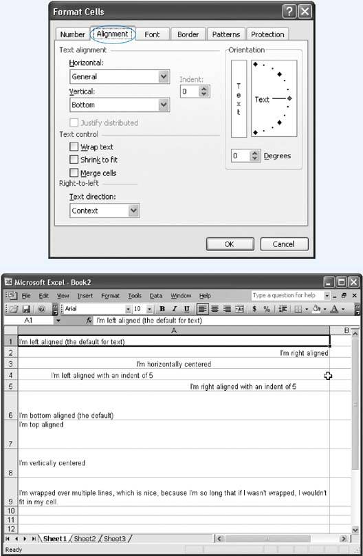
Vertical alignment controls the position of content between a cell's top and bottom border. Vertical alignment becomes important only if you enlarge a row's height so that it becomes taller than the contents it contains. To change the height of a row, click the bottom edge of the row header (the numbered cell on the left side of the worksheet), and drag it up or down. As you resize the row, the content stays fixed at the bottom. The vertical alignment setting lets you adjust the cell content's positioning. Excel gives you the following vertical alignment choices, some of which are shown in Figure 4-7, bottom: Top. Top indicates that the first line of text starts at the top of the cell. Center. Center tells Excel to center the block of text between the top and bottom border of the cell. Bottom. Bottom indicates that the last line of text ends at the bottom of the cell. If the text doesn't fill the cell exactly, Excel adds some padding to the top. Justify. Justify is the same as Top for a single line of text. If you have more than one line of text, Excel increases the spaces between each line so that the text fills the cell completely from the top edge to the bottom edge. Distributed. This option is the same as Justify for multiple lines of text. If you have a single line of text, Distributed creates the same result as Center.
If you have a cell containing a large amount of text, you can increase the row's height so you can display multiple lines. Unfortunately, you'll notice that enlarging a cell doesn't automatically cause the text to flow into multiple lines and fill the newly available space. But there's a simple solution: just turn on the "Wrap text" checkbox (on the Alignment tab of the Format Cells dialog box). Now, long passages of text will flow across multiple lines. You can use this option in conjunction with the vertical alignment setting to control whether Excel centers a block of text or lines it up at the bottom or top of the cell. Another option is to explicitly split your text into lines. Whenever you want to insert a line break, just press Alt+Enter and start typing the new line. FREQUENTLY ASKED QUESTION
Fitting More Text into a Cell | I'm frequently writing out big chunks of text that I'd love to scrunch into a single cell. Do I have any options other than text wrapping? Yes. If you need to store a large amount of text in one cell, text wrapping is a good choice. But it's not your only option. You can also shrink the size of the text or merge multiple cells, both of which you can do from the Alignment tab of the Format Cells dialog box. To shrink a cell's contents, select the "Shrink to fit" checkbox. Be warned, however, that if you have a small column that doesn't use wrapping, this option can quickly reduce your text to vanishingly small proportions. 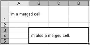 Joining multiple cells together removes the cells' shared borders and creates one mega-sized cell. Usually, you'll use joining (or merging) to accommodate a large amount of content that can't fit in a single cell (like a long title that you want to display over every column). For example, if you merge cells A1 and B1, you'll end up with a single cell named A1 that stretches over the full width of the A and B columns, as shown at bottom left. To merge cells, select the cells you want to join, choose Format  Cells, and on the Alignment tab, turn on the "Merge cells checkbox. There's no limit to how many cells you can merge. (In fact, you can actually convert your entire worksheet into a single cell if you want. Whee.) And if you change your mind, don't worryyou simply need to select the single merged cell, choose Format Cells again, and clear the checkmark in the "Merge cells checkbox to redraw the original cells. Cells, and on the Alignment tab, turn on the "Merge cells checkbox. There's no limit to how many cells you can merge. (In fact, you can actually convert your entire worksheet into a single cell if you want. Whee.) And if you change your mind, don't worryyou simply need to select the single merged cell, choose Format Cells again, and clear the checkmark in the "Merge cells checkbox to redraw the original cells. |
Tip: After you've expanded a row, you can shrink it back by double-clicking the bottom edge of the row header. If you haven't turned on text wrapping, double-clicking shrinks the row back to its standard single-line height.
Finally, the Alignment tab lets you rotate content in a cell up to 180 degrees, as shown in Figure 4-7. You can set the number of degrees you want your text to rotate in either of two ways: by dragging the "arm" that appears on the right side of the Alignment tab or by clicking the Degrees box. Rotating cell content automatically changes the size of the cell (see Figure 4-8). Usually, you'll see it become narrower and taller to accommodate the rotated content. Figure 4-8. If you set your text orientation at 15 Degrees (see Orientation box in Figure 4-7, set at 0 Degrees), the text would print at an angle, as shown in the headings here. The rotated text may look a little blurry on the screen, but it will look much clearer when printed. 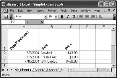
Tip: Thanks to Excel's handy Redo feature, you can repeatedly apply a series of formatting changes to different cells. After you make your changes in the Format Cells dialog box, simply select the new cell you want to format in the same way and then hit Ctrl+Y to repeat the last action.
4.2.2. Fonts and Color As in almost any Windows program, you can customize text in Excel, applying a dazzling assortment of colors and fancy typefaces. You can do everything from enlarging headings to shrinking footnotes. Other settings you can change include: The font style. (For example, Arial, Times New Roman, or something a little more shocking, like Futura Extra Bold). Arial is the standard font for new worksheets. The font size, in points. Out of the box, Excel uses point size 10, but you can choose anything from a minuscule 1-point to a monstrous 409-point. Excel automatically enlarges the row height to accommodate the font. Various font attributes, like italics, underlining, and bold. Some fonts have complementary italic and bold typefaces, while others don't (in which case Windows will use its own algorithm to embolden or italicize the font). The font color. This option controls the color of the text. (The next section, "Borders and Patterns") covers how to change the color of the entire cell.)
To change font settings, first highlight the cells you want to format, choose Format Cells, and then click the Font tab (Figure 4-9). The Formatting toolbar also provides a number of shortcuts that let you quickly change certain font settings, including font, size, color, and attributes like boldface and italics. The Formatting toolbar sits in the row just under Excels main menu; you can find out more about it on Section 4.3.1. (Truth be told, the formatting toolbar is way more convenient for setting fonts, because its drop-down menu shows a long list of font names, whereas the font list in the Format Cells dialog box is limited to showing an impossibly restrictive four fonts at a time. Scrolling through that cramped space is more than a little maddening.) Not all fonts are equal. When displaying dataespecially numberssans-serif fonts are usually clearer and look more professional than serif fonts. (Serif fonts have little embellishments, like tiny curls, on the ends of the letters; sans-serif fonts don't.) Arial, the default spreadsheet font, is a sans-serif font. The font used for the body text of this book, Adobe Minion, is clearly a serif font, which works best for large amounts of text. Figure 4-9. You can apply an exotic font through the Format Cells dialog box. 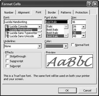
Note: No matter what font you apply, Excel, thankfully, always displays the cell contents in the eye-friendly Arial font in the Formula bar. That makes things easier if you happen to be working with cells that have been formatted to use graphically complex or large fonts.
Tip: Excel always assumes you want your worksheet font to be Arial unless you tell it otherwise. To change the font setting, select Tools Options and then click the General tab. Next to the "Standard font label are two drop-down menus where you can set the standard font and font size. The font you choose won't apply to existing worksheets, but Excel will use it every time you create a new worksheet.
4.2.2.1. Special characters Most fonts contain not only digits and the common letters of the alphabet, but also some special symbols that you can't type directly on your keyboard. One example is the copyright symbol ©, which you can insert into a cell by typing in the text (C) and letting AutoCorrect do its work. Other symbols, however, aren't as readily available. One example is the special arrow character, . To use this symbol, youll need the help of the Wingdings font.
Note: Wingdings isn't the only font with special characters (although it does have a really great selection). You can insert extended characters from any font by selecting the name of the font from the Symbol dialog's drop-down list. (Extended characters are mostly non-English letters like Arabic or Hebrew letters.)
Wingdings is a special font included with Windows that's made up entirely of symbols like arrows, smiley faces, and zodiac signs, none of which are found in standard fonts. You can try to apply the Wingdings font on your own, but it won't be easy, because you won't know which character to press on your keyboard to get the symbol you want. A better choice is to use Excel's Symbol dialog box. Simply follow these steps: Choose Insert Symbol from the menu. Figure 4-10. The Symbol dialog box lets you insert special characters. 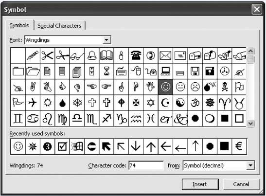 Choose the font that has the special character you want to insert. In the Font box, scroll down and select Wingdings (if it's not already selected). In addition, you can find a few predefined special characters, like the copyright symbol, on the Special Characters tab of the Symbol dialog box. Select the character, and then click Insert. Alternatively, if you need to insert multiple special characters, just double-click each one; doing so inserts each symbol right next to each other in the same cell without having to close the window.
When Excel inserts a character from the Symbol dialog box, it doesn't change the font for the cell. What you'll actually end up with is a cell that has two fontsone for the symbol character and one for the rest of your text. This approach works perfectly well, but it can cause some confusion. For example, if you apply a new font to the cell after inserting a special character, Excel adjusts the entire contents of the cell to use the new font, and your symbol will change into the corresponding character in the new font (which usually isn't what you want). These problems aren't unique to using symbols; they can crop up any time you deal with a cell that has more than one font.
Note: If you look at the cell contents in the Formula bar, you'll always see the cell data in the standard Arial font. That means, for example, that your Wingdings symbol won't appear as the icon that shows up in your worksheet. Instead, you'll see an ordinary letter or some type of extended non-English character, like æ.
4.2.3. Borders and Patterns The best way to call attention to important information isn't to change fonts or alignment. Instead, place borders around key cells or groups of cells and use shading to highlight important columns and rows. Excel provides dozens of different ways to outline and highlight any selection of cells.
Note: Removing a worksheet's gridlines, as shown in Figure 4-11, lets you focus visually on any custom borders you've added (or are about to add). To remove a worksheet's gridlines, select Tools Options. From the Options dialog box that appears, select the View tab and then turn off the checkmark next to the Gridlines checkbox. (This grid-removing procedure affects only the current file and wont apply to new spreadsheets.)
Once again, the trusty Format Cells dialog box is your control center. Just follow these steps: Select the cells you want to fill or outline. Your selected cells appear highlighted.
Note: The Gridlines setting has no effect on whether or not Excel adds the worksheet gridlines to a printout. You can control whether your borders appear in printed versions of your worksheet through the Page Setup setting, as described on Section 6.2.2.4.
Figure 4-11. This worksheet has no gridlines. 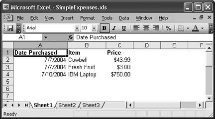 Select Format Cells, or just right-click the selection and choose Format Cells. Head directly to the Border tab. (If you don't want to apply any borders, skip straight to step 4.) Applying a border is a multistep process (see Figure 4-12). Begin by choosing the line style you want (dotted, dashed, thick, double, and so on), followed by the color (Automatic picks black). Both these options are on the right side of the tab. Next, choose where your border lines are going to appear. The Border box (where the word "Text" appears four times) functions as a nifty, interactive test canvas that shows you where your lines are going to appear. To make your selection, you can either click one of the eight Border buttons (which contain a single bold horizontal, vertical, or diagonal line), or you can click directly inside the Border box. If you change your mind, clicking a border line will make it disappear. For example, if you want to apply a border to the top of your selection, click the top of the Border box. If you want to apply a line between columns inside the collection, click between the cell columns in the Border box. The line appears indicating your selection. Figure 4-12. Follow the numbered steps in this figure to choose the line style and color, and then apply the border. 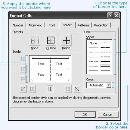
Tip: The Border tab also provides two shortcuts in the Presets region of the tab. If you want to apply a border style around your entire selection, select Outline after choosing your border style and color. Choose Inside to apply the border between the rows and columns of your selection. Make a mistake? Select None to start over.
Click the Patterns tab. Here you can select the color and pattern of any shading you want to add to the cells in the selection (see Figure 4-13). Adding a color and pattern to selected cells is simpler than choosing borders. All you need to do is select the color you want and then, if you want, choose a pattern. You can tell Excel to draw the pattern in a different color (click Pattern, and then choose a color) and even tell it to include diagonal lines, a grid, dots, or the tight checker-board shown in Figure 4-13. Figure 4-13. Choose your color and pattern on this tab. 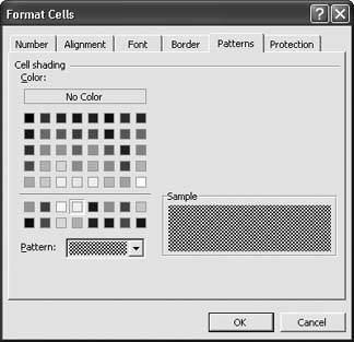
Note: In general, patterns obscure text, and you shouldn't apply them to cells that have content. Simple color fills tend to work better, provided you use light colors that will allow text or numbers to remain legible.
Click the No Color box to clear any current color or pattern in the selected cells. Click OK to apply your changes. If you don't like the modifications you've just applied, you can roll back time with a quick application of the Edit Undo command.
GEM IN THE ROUGH
Your Favorite Colors | Excel gives you a fairly narrow set of color choices for fonts, borders, and fills, which you can find by choosing Tools Options and then clicking the Color tab. The 56 colored boxes are your basic choices. You can, however, alter those colors. Select one of the color boxes and then click the Modify button. Youll see a more extensive dialog box that lets you pick an exact shade. 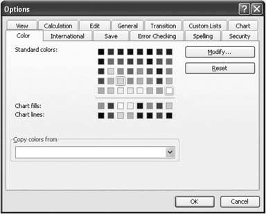 Bear in mind that you can't tweak any of the colors while you're formatting a cell. Instead, you need to set the color beforehand. Also, although Excel lets you modify colors, there's no way to create extra colors in a worksheet. Color settings are specific to a single workbook file, but you can copy them from one file to another. To do so, just open both workbooks at once and then, in the workbook where you want to place the copied colors, choose Tools Options. Click the color tab and then, in the "Copy colors from list, find the name of the workbook that has the colors you want to copy. Excel refreshes the set of colors immediately. You can also click Reset to return your color settings to Excel's standard choices. |
|