Chapter Eleven. Signal Averaging
Eleven Signal Averaging
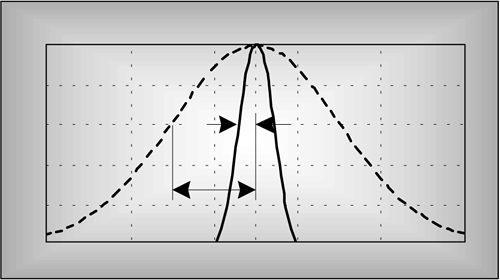
How do we determine the typical amount, a valid estimate, or the true value of some measured parameter? In the physical world, it's not so easy to do because unwanted random disturbances contaminate our measurements. These disturbances are due to both the nature of the variable being measured and the fallibility of our measuring devices. Each time we try to accurately measure some physical quantity, we'll get a slightly different value. Those unwanted fluctuations in a measured value are called noise, and digital signal processing practitioners have learned to minimize noise through the process of averaging. In the literature, we can see not only how averaging is used to improve measurement accuracy, but that averaging also shows up in signal detection algorithms as well as in low-pass filter schemes. This chapter introduces the mathematics of averaging and describes how and when this important process is used. Accordingly, as we proceed to quantify the benefits of averaging, we're compelled to make use of the statistical measures known as the mean, variance, and standard deviation.
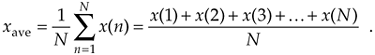
In digital signal processing, averaging often takes the form of summing a series of time-domain signal samples and then dividing that sum by the number of individual samples. Mathematically, the average of N samples of sequence x(n), denoted xave, is expressed as
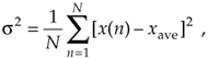
(What we call the average, statisticians call the mean.) In studying averaging, a key definition that we must keep in mind is the variance of the sequence s2 defined as
Equation 11-2
Equation 11-2'

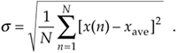
As explained in Appendix D, the s2 variance in Eqs. (11-2) and (11-2') gives us a well defined quantitative measure of how much the values in a sequence fluctuate about the sequence's average. That's because the x(1) – xave value in the bracket, for example, is the difference between the x(1) value and the sequence average xave. The other important quantity that we'll use is the standard deviation defined as the positive square root of the variance, or
Equation 11-3
To reiterate our thoughts, the average value xave is the constant level about which the individual sequence values may vary. The variance s2 indicates the sum of the magnitudes squared of the noise fluctuations of the individual sequence values about the xave average value. If the sequence x(n) represents a time series of signal samples, we can say that xave specifies the constant, or DC, value of the signal, the standard deviation s reflects the amount of the fluctuating, or AC, component of the signal, and the variance s2 is an indication of the power in the fluctuating component. (Appendix D explains and demonstrates the nature of these statistical concepts for those readers who don't use them on a daily basis.)
We're now ready to investigate two kinds of averaging, coherent and incoherent, to learn how they're different from each other and to see under what conditions they should be used.
URL http://proquest.safaribooksonline.com/0131089897/ch11
| Amazon | ||
