Training Algorithms

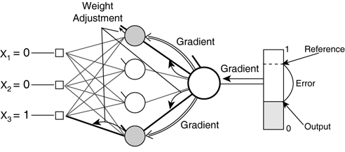
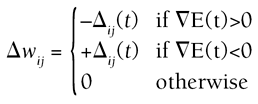
The mathematical background in MLPs does provide one advantage: They can be trained. Just like for perceptrons with single layers, the task of training an MLP is fundamentally about numeric optimization. The ideal value of each weight must be found to minimize the output error. This is slightly more challenging because it's harder to determine the necessary adjustment to correct the weights (because the gradient of the error cannot be computed directly). This explains the additional complexity of the training algorithms.

Back Propagation

Backprop is the process of filtering the error from the output layer through the preceding layers. This was developed because of problems with the original perceptron training algorithms: They were unable to train the hidden layers. Back propagation is the essence of most MLP learning algorithms, because it allows the gradient to be determined in each weight (so they can be optimized).

Informal Explanation

For the last layer, the error of the output is immediately available, computed as the difference between the actual output and the desired output. Using the exact same principles as for the perceptron, the gradient of the error in each weight can be found. The gradient descent algorithms can use the slope of the error to adjust the weights in the last layer.

For hidden layers, the error is not immediately available because there is no reference to compare the output to! Instead, we notice that some hidden neurons are connected to output neurons whose error is known. The error in the output must partly originate from the hidden neurons. By propagating the error backward through the neural network, it's essentially possible to distribute the blame for the error on predecessor neurons.

This back-propagation process, shown in Figure 19.5, propagates the error gradient. The error gradient of a hidden unit is the weighted sum of the error gradients in the output units. The weights of the connections determine hidden error gradient from known processing units.

Figure 19.5. Backward propagation of the error throughout the layers, distributed from the output via the weighted connections.

This can be understood as a recursive definition of the error gradient. No matter how many layers are present, we can work backward from the outputs and compute all the error gradients in the processing units. Then, using the same technique as for perceptrons, we can compute the gradient in each of the individual weights. Steepest descent or any other gradient based optimization is then applied to the weights to adjust them accordingly.

Formal Proof

This section is only intended for those with an interest in the underlying details of training. We're trying to find the derivative of the error with respect to the weight connecting unit i to unit j, denoted E/w_ij. This can be split into three parts using the chain rule (as done implicitly for the proof on the perceptron):

We start with the third term on the right, the derivative of the net sum of unit j with respect to the weight z_j/w_ij. This turns out to be the output y_i of the previous unit i (or the network input for the first layer):

The second term y/z_j expresses the gradient of unit j's output with respect to the net sum. This is defined by the activation function, so its derivative needs to be taken:

Finally, the first right-side term is left E/y_j, representing the gradient of the error in terms of the unit's output. This is straightforward for those units in the output layer (as with standard perceptrons):

For those units j that are not connected straight to the MLP's output, the term is computed recursively in terms of the units k that are along the connection toward the output. It's the sum () of the error gradient relative to the output of k E/y_k, multiplied by the gradient output relative to the net sum y_k/z_k, and the weight between j and k w_jk.

In general, it is useful to use an easier notation to implement the algorithm. If we define the following

Then the gradient of the error relatively to the net sum d_j can be computed depending on its position in the network:

This emphasizes the need for a backward-propagation process, where d_j is computed for each unit of each layer depending on the previous unit's k.

Backprop Algorithm

There is a simple training algorithm based on the application of these equations; incremental training is applied to a set of examples. The method is known as backprop, but in fact the actual backward propagation is only one part of the process. Back propagation is the first stage of the algorithm, used to compute the gradients in each of the neurons (and then the weights later).

The outline in Listing 19.2 is at the core of all the gradient-based techniques, because it actually computes the gradient. Now the second stage of the backprop algorithm performs steepest descent to the weights (see Listing 19.3). (This is where learning happens.)

Listing 19.2 Backward-Propagation Algorithm Used to Compute the Gradient of the Error in Each of the Units

 # compute the gradient in the units of the first layer for each unit j in the last layer delta[j] = deriv_activate(net_sum)     * (desired[j] - output[j]) end for # process the layers backwards and propagate the error gradient for each layer from last-1 down to first      for each unit j in layer           total = 0           # add up the weighted error gradient from next layer           for each unit k in layer+1                total += delta[k] * weights[j][k]           end for      delta[j] = deriv_activate(net_sum) * total      end for end for 

Listing 19.3 Steepest Descent on the Error Gradient in Each of the Weights

 for each unit j      for each input i           # adjust the weights using the error gradient computed           weight[j][i] += learning_rate * delta[j] * output[i]      end for end for 

The rule used to compute the step for each weight Dw_ij is known as the generalized delta rule, an extension of the delta rule used to train standard perceptrons. The learning rate h is a small constant set by the engineer. d_j is the gradient of the error of unit j relative to the net sum z_j. This is used to compute the necessary change in the weights to perform gradient descent.

Quick Propagation

Quickprop is a batch technique based on a combination of ideas. First, it exploits the advantages of locally adaptive techniques that adjust the magnitude of the steps based on local parameters (for instance, the nonglobal learning rate). Second, knowledge about the higher-order derivative is used (such as Newton's mathematical methods). In general, this allows a better prediction of the slope of the curve and where the minima lies. (This assumption is satisfactory in most cases.)

Quickprop Theory

The procedure to update the weights is very similar to the standard backprop algorithm. The gradient of the error in each weight is needed, denoted E(t). This is the gradient for all the training samples because quickprop is a batch update algorithm:

This value is necessary for the current epoch t (a learning period) and the previous one t-1 denoted E(t 1). The same applies for the weight update step w_ij(t) and w_ij(t 1). Then, the weight update can be determined as follows:

In practice, this proves much more efficient than the standard backprop on many problems. However, some of the assumptions about the nature of the slope can prove problematic in other cases. This really depends on each problem, and can be tested by comparing this algorithm's performance with the two others.

Implementing Quickprop

To implement this, two more arrays are needed for the step and the gradient, remembering values from the previous iteration. Because it's a batch algorithm, all the gradients for each training sample are added together. The backprop algorithm can achieve this by accumulating d_j at each iteration. These values will get reset only when a new epoch starts (that is, when the iteration over all the samples restarts).

The second part of the backprop algorithm is replaced; we use the new weight update rule rather than steepest descent (see Listing 19.4).

Listing 19.4 The Weight Update Procedure as Used by the Quick-Propagation Algorithm

 for each unit j      for each input i           # compute gradient and step for each weight           new_gradient[j][i] = -delta[j] * input[i]           new_step[j][i] = new_gradient[j][i] / (old_gradient[j][i] new_gradient[j][i])                 * old_step[j][i]           # adjust the weight           weight[j][i] += new_step[j][i]           # store values for the next computation           old_step[j][i] = new_step[j][i]           old_gradient[j][i] = new_gradient[j][i]      end for end for 

Given a working backprop algorithm, the quickprop variation does not take long to implement and test.

Resilient Propagation

RProp is another batch algorithm that updates the weights only after all the training samples have been seen [Riedmiller93]. The key idea is that the size of the step used to update the weights is not determined by the gradient itself, which removes the major problems associated with steepest descent techniques.

RProp Theory

The algorithm introduces the concept of update value D_ij, which is used to determine the step Dw_ij. It's important not to confuse the two, and the notation chosen by Riedmiller and Braun does not help. The update value is used to determine the step:

This is relatively intuitive to understand. If the slope goes up, we adjust the weight downward (first case). Conversely, the weight is adjusted upward if the gradient is negative (second case). If there is no slope, we must be in a minima, so no step is necessary (third case). This equation is needed to compute the new update value:

h⁺ and h are constants defined such that 0<h <1<h⁺. Informally, the size of the step is increased (multiplied by h⁺) if the gradient maintains the same direction (first case). The step size is decreased (multiplied by h ) if the gradient changes sign (second case). Otherwise, the step size is left untouched if the gradient is 0.

Implementing RProp

Once again, we need extra arrays with the previous error gradients as well as the previous update value for each weight. As a batch algorithm too, the first loop to compute the sum of the gradients is the same as quickprop's. Then, the second stage of the algorithm is applied to update the weights, as shown in Listing 19.5.

Listing 19.5 The Weight Update Procedure Behind the Resilient-Propagation Algorithm

 for each unit j      for each input i           # first determine the gradient in the neuron           new_gradient[j] = delta[j] * input[i]           # analyze gradient change to determine size of update           if new_gradient[j] * old_gradient[j] > 0 then                new_update[j][i] = nplus * old_update[j][i]           else if new_gradient[j] * old_gradient[j] < 0 then                new_update[j][i] = nminus * old_update[j][i]           else                new_update[j][i] = old_update[j][i]           # determine which direction to step in           if new_gradient[j] > 0 then                step[j][i] = -new_update[j][i]           else if new_gradient[j] < 0 then                step[j][i] = new_update[j][i]           else step[j][i] = 0           # adjust weight and store values for next iteration           weight[j][i] += step[j][i]           old_update[j][i] = new_update[j][i]           old_gradient[j][i] = new_gradient[j][i]      end for end for 

This is slightly trickier to implement, but is still classified as a simple task after backprop has been written!