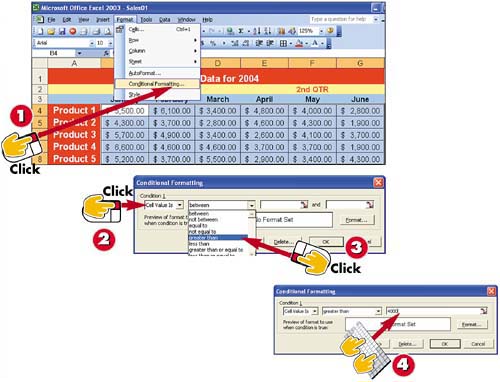
Select the cells to which you want to apply conditional formatting, then open the Format menu and select Conditional Formatting.
In the Conditional Formatting dialog box, keep the default Condition 1 as Cell Value Is (use Formula Is to indicate a specific formula).
Display the second drop-down list to select the type of condition (for example, greater than).
Type the value of the condition (the number that the cells must be "greater than").
INTRODUCTION
You might want the formatting of a cell to depend on the value it contains. For this, you use conditional formatting, which lets you specify conditions that, when met, cause the cell to be formatted in the manner defined for that condition. If none of the conditions are met, the cell keeps its original formatting. For example, you can set a conditional format such that, if sales for a particular month were above $4,000, the data in the cell is bold and red.
TIP
Painting onto Other Cells
You can copy the conditional formatting from one cell to another. To do so, click the cell whose formatting you want to copy. Then click the Format Painter button. Finally, drag over the cells to which you want to copy the formatting.
Click the Format button to set the format to use when the condition is met.
Click the options you want to set in the Format Cells dialog box (for example, Purple in the Color field and Bold in the Font style list), and click OK.
Click OK in the Conditional Formatting dialog box.
Excel applies the formatting to any cells that meet the condition you specified.
TIP
When to Use Conditional Formatting
Use conditional formatting to draw attention to values that have different meanings, depending on whether they are positive or negative, such as profit and loss values.