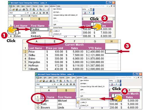
Click the cell to the right of and below the area you want to freeze. (Typically, this is cell B2 if your main header row is Row 1 and your main column is Column A.)
Open the Window menu and select Freeze Panes.
Move through the worksheet using the arrow keys on your keyboard. Frozen Row 1 and Column A enables you to view your data without losing sight of the titles.
Open the Window menu and select Unfreeze Panes to unfreeze the columns and rows.
INTRODUCTION
Many of your worksheets might be large enough that you cannot view all the data onscreen at the same time. In addition, if the worksheet contains row or column titles and you scroll down or to the right, some of the titles are too far to the top or left of the worksheet for you to see.
TIP
Splitting a Worksheet
By splitting a worksheet, you can scroll independently into different horizontal and vertical parts of a worksheet. This is useful if you want to view different parts of a worksheet or copy and paste between different areas of a large worksheet. Simply unfreeze the panes, and then open the Window menu and select Split. You can move the split bars by clicking and dragging them as necessary.