6.11. PRINCIPLES OF IMPLEMENTATION | Parallel Computing on Heterogeneous Networks (Wiley Series on Parallel and Distributed Computing)

6.10. A SIMPLE HETEROGENEOUS ALGORITHM SOLVING A REGULAR PROBLEM

An irregular problem is characterized by some inherent coarse-grained or large-grained structure. This structure implies a quite deterministic decomposition of the whole problem into a relatively small number of subtasks, which are of different size and can be solved in parallel. Correspondingly a natural way of decomposing the whole program, which solves the irregular problem on a network of computers, is by a set of parallel processes solving the subtasks and altogether interacting via message passing. As sizes of these subtasks differ, the processes perform different volumes of computation. Calculation of the mass of a metallic construction welded from N heterogeneous rails is an example of an irregular problem.

The most natural decomposition of a regular problem is a large number of small identical subtasks that can be solved in parallel. As those subtasks are identical, they are all of the same size. Multiplication of two n n dense matrices is an example of a regular problem. This problem is naturally decomposed into n² identical subtasks, each of which is to compute one element of the resulting matrix.

An efficient solution on a heterogeneous network of computers would transform the problem into an irregular problem, whose structure is determined by the structure of the executing network rather than the structure of the regular problem itself. This way the whole regular problem is decomposed into a set of relatively large subproblems, each made of a number of small identical subtasks stuck together. The size of each subproblem, that is, the number of elementary identical subtasks constituting the subproblem, depends on the speed of the processor, on which the subproblem will be solved.

Correspondingly the parallel program that solves the problem on the heterogeneous network of computers is a set of parallel processes, each handling one subproblem on a separate physical processor and altogether interacting via message passing. The volume of computations performed by each of these processes should be proportional to its speed.

In Section 5.1 we considered a simple heterogeneous parallel algorithm of matrix-matrix multiplication on a heterogeneous network of computers as well as its implementation in HPF 2.0. Let us now consider a much similar algorithm of parallel multiplication on a heterogeneous network of matrix A and the transposition of matrix B, performing matrix operation C = A B^T, where A, B are dense square n n matrices.

This algorithm can be summarized as follows:

Each element in C is a square r r block and the unit of computation is the computation of one block, that is, a multiplication of r n and n r matrices. For simplicity we assume that n is a multiple of r.
The A, B, and C matrices are identically partitioned into p horizontal slices, where p is the number of processors performing the operation. There is one-to-one mapping between these slices and the processors. Each processor is responsible for computing its C slice.
Because all C blocks require the same amount of arithmetic operations, each processor executes work proportional to the number of blocks that are allocated to it, hence, proportional to the area of its slice. To balance the load of the processors, the area of the slice mapped to each processor is proportional to its speed (see Figure 6.1).

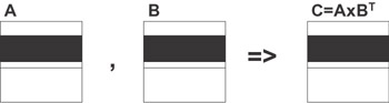
Figure 6.1: Matrix operation C = A x B^T with matrices A, B, and C unevenly partitioned in one dimension. The slices mapped onto a single processor are shaded in black.
At each step a row of blocks (the pivot row) of matrix B, representing a column of blocks of matrix B^T, is communicated (broadcast) vertically, and all processors compute the corresponding column of blocks of matrix C in parallel (see Figure 6.2).

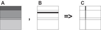
Figure 6.2: One step of parallel multiplication of matrices A and B^T. The pivot row of blocks of matrix B (shown slashed) is first broadcast to all processors. Then each processor computes, in parallel with the others, its part of the corresponding column of blocks of the resulting matrix C.

The following mpC program implements this algorithm:

#include <stdio.h> #include <stdlib.h> #include <mpc.h> void Partition(), SerialAxBT(); nettype ParallelAxBT(int p, int d[p]) {    coord I = p;    node { I>=0: d[I]; };    parent [0]; }; int [*]main(int [host]argc, char **[host]argv) {    repl int n, r, p, *d;    repl double *speeds;    n = [host]atoi(argv[1]);    r = [host]atoi(argv[2]);    /* Run a test code in parallel by all physical processors */    /* to refresh information about their speeds */    {       repl double a[r][n], b[r][n], c[r][n];       repl int i, j;       for(i=0; i<r; i++)          for(j=0; j<n; j++)          {             a[i][j] = 1.0;             b[i][j] = 1.0;       }    recon SerialAxBT((void*)a, (void*)b, (void*)c, r, n); } /* Detect the total number of physical processors */ p = MPC_Get_number_of_processors(); speeds = calloc(p, sizeof(double)); d = calloc(p, sizeof(int)); /* Detect the speed of the physical processors */ MPC_Get_processors_info(NULL, speeds); /* Calculate the number of rows of the resulting matrix */ /* to be computed by each processor */ Partition(p, speeds, d, n, r); {    net ParallelAxBT(p, d) w;    int [w]myn;    myn = ([w]d)[I coordof w];    [w]:    {       double A [myn/r][r][n], B[myn/r][r][n],        C[myn/r][r][n];       repl double Brow[r][n];       int i, j, k;       for(i=0; i<myn/r; i++)          for(j=0; j<r; j++)             for(k=0; k<n; k++)             {               A[i][j][k] = 1.0;               B[i][j][k] = 1.0;             } {    repl int PivotNode=0, RelPivotRow, AbsPivotRow;    for (AbsPivotRow=0, RelPivotRow=0, PivotNode=0;       AbsPivotRow < n;       RelPivotRow += r, AbsPivotRow += r)    {       if(RelPivotRow >= d[PivotNode])       {          PivotNode++;          RelPivotRow = 0;       }       Brow[] = [w:I==PivotNode]B[RelPivotRow/r][];       for(j=0; j<myn/r; j++)          SerialAxBT((void*)A[j][0], (void*)Brow[0],                (void*)(C[j][0]+AbsPivotRow), r, n);             }          }       }    }    free(speeds);    free(d); } void SerialAxBT(double *a, double *b, double *c, int r, int n) {    int i, j, k;    double s;    for(i=0; i<r; i++)    for(j=0; j<r; j++)    {       for(k=0, s=0.0; k<n; k++)          s += a[i*n+k]*b[j*n+k];       c[i*n+j]=s;    } } void Partition(int p, double *weight, int *d, int n, int r) {    int rows, distributed_rows, i;    double total_weight;    rows = n/r;    for(i=0, total_weight=0.0; i<p; i++)       total_weight += weight[i];    for(i=0, distributed_rows=0; i<p; i++)    {       d[i] = (int)(weight[i]/total_weight*rows);       distributed_rows += d[i];    }       for(i=0; i<p && distributed_rows!=rows; i++, distributed_rows++)       d[i]++;    if(distributed_rows!=rows)       d[0] += rows-distributed_rows;    for(i=0; i<p; i++)       d[i] *= r; }

In this program the network type ParallelAxBT describes two features of the implemented algorithm of parallel matrix multiplication:

The number of involved parallel processes.
The relative volume of computations to be performed by each of the processes.

The definition of ParallelAxBT declares that an mpC network of p abstract processors will perform the algorithm. It is supposed that the ith element of vector parameter d is just the number of rows in the C slice mapped to the ith abstract processor of the mpC network. Thus the node declaration specifies relative volumes of computations to be performed by the abstract processors.

Network w is defined so that

one-to-one mapping would occur between its abstract processors and physical processors of the executing network, and
the volume of computation to be performed by each abstract processor would be proportional to the speed of the physical processor running the abstract processor.

To achieve this, the program first detects the number of physical processors that execute the program. This is achieved by calling the nodal library function MPC_Get_number_of_processors. The function is called by all processes of the program in parallel. So after this call the value of all projections of replicated variable p will be equal to the total number of physical processors executing the program.

Then the program detects the speeds of the physical processors by calling the nodal library function MPC_Get_processors_info. The function returns in array speeds the latest information about the speed of processors, which the programming system has received. In this case it will be the speed demonstrated by the processors during execution of the code specified in the recon statement. The code just multiplies the test r x n and n x r matrices with a call to function SerialAxBT.

Note that computations performed in this program mainly fall into calls to function SerialAxBT, each of which multiplies two r x n and n x r matrices. Therefore, after the call to function MPC_Get_processors_info, the value of speeds [i] will be very close to the speed of the ith physical processors demonstrated during the execution of the program (i = 0,...,p-1).

The test code used to estimate the speed of processors must match well the computations performed by the program. For example, if we used mutiplication of two 200 x 200 matrices in the program above for estimation of the speed of processors, the resulting estimation would typically be much less accurate. The reason is that multiplication of 10 x 4000 and 4000 x 10 matrices causes more intensive data swapping between different levels of the memory hierarchy than multiplication of two 200 x 200 matrices. As a result, despite these two matrix operations performing the same amount of arithmetic operations, the amount of memory access operations will be different. So the underlying computations will be different as well.

click to expand

Finally, the program defines an mpC network, w, which consists of as many abstract processors as many the physical processors are involved in the execution of the program. The relative volume of computations to be performed by the ith abstract processor of network w is specified to be proportional to the speed of the ith physical processor. Therefore any conforming implementation of mpC will map the ith abstract processor of w to a process running on the ith physical processor, just because this is the very mapping that makes the speed of each abstract processor proportional to the volume of computation that the abstract processor performs.

The rest of the program code describes the parallel matrix multiplication on network w itself. First of all, each abstract processor of w computes the number of rows in the C slice to be computed by the processor, and stores this number in variable myn. Then the program defines the distributed arrays A, B, and C to store matrices A, B, and C respectively. The horizontal slice of matrix A mapped to each abstract processor of network w will be stored in its projection of array A. Note that projections of the distributed array A are of different shapes depending on the size of the A slice mapped to one or another processor. The same is true for distributed arrays B and C.

The program also defines a replicated array, Brow, to store the pivot row of matrix B. All projections of array Brow are of the same shape. After that, a nested for-loop executed by all abstract processors of network w in parallel initializes distributed arrays A and B.

Finally, the main for-loop of the program describes n/r steps of the matrix multiplication algorithm. At each step, assignment

Brow[] = [w:I==PivotNode]B[RelPivotRow/r][]

broadcasts a row of blocks (the pivot row) of matrix B, representing a column of blocks of matrix B^T, to all abstract processors of network w, where it is stored in array Brow. Then all of the abstract processors compute the corresponding column of blocks of matrix C in parallel.