Measures

Now that we have a real live cube in captivity, we can study its basic parts and look at some of its more advanced features. We begin with measures. Measures provide the actual information that the users of our cubes are interested in. Measures are the bits of numerical data that we need to aggregate. As we saw in the Cube Wizard, measures come from the fields in the fact tables in the data mart.

SQL Server 2005 Analysis Services provides us with a number of features for managing measures. We can even create new measures that don't exist in the data mart. We can also control the aggregation of the measures along our dimensions.

Measure Groups

In SQL Server 2005 Analysis Services, measures do not exist on their own inside cubes. Instead, they are clustered together and managed in groupings. These groupings are called measure groups. Each measure group in a cube corresponds to a table in the data source view. This table is the measure group's source for its measure data. The measure group is said to be bound to this table. Each record in the table becomes a different member of the measure group.

In the Max Min Manufacturing DM cube created by the Cube Wizard, there is a single measure group called Manufacturing Fact. This measure group contains the Accepted Products, Rejected Products, and Elapsed Time for Manufacture measures. This measure group is bound to the ManufacturingFact table in the data source view.

Measure Groups and Dimensions

Previously, we discussed how dimensions are used to aggregate measures. For this aggregation to take place, the dimensions in a cube must be somehow related to the measures. When we created our data marts, this was done using a foreign key field in the measure or fact table that linked to primary key fields of our dimension tables. In the cube itself, we do the same thing by creating relationships between the measure groups and the dimensions.

At first, this may seem a bit strange. As we have discussed cubes conceptually in previous chapters, we have always talked about measures being related to dimensions, with no talk of measure groups. When we query the data from our cubes, we use dimensions as if they were directly related to measures. However, if you consider the underlying architecture, this makes perfect sense.

In our data mart, we have multiple measures in a single record of our fact table. In the Manufacturing data mart, the Accepted Products, Rejected Products, and Elapsed Time for Manufacture treasures are present in each record. The record also contains the foreign key fields linking it to the lowest-level dimension tables in each of the hierarchies. Again, in the Manufacturing data mart, these are DimProduct, DimBatch, and DimMachine (along with the time dimension that is created virtually from the DateOfManufacture field).

All of the measures in the ManufacturingFact record (a single row of data) depend on all of the foreign key fields in that record. Therefore, if a given Accepted Products measure and Rejected Products measure reside in the same record, it is impossible for them to relate to two different records in the DimProduct table. See Figure 8-8. Only one foreign key field in their record can be used to link to the DimProduct table, so they must both link to the same product. That's the way well-normalized relational databases work.

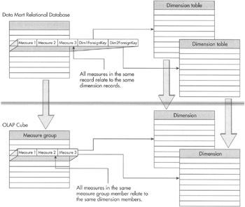
Figure 8-8: Measure groups and dimensions

We just said that measure groups correspond to a table in the data source view. Just as all of the measures in a given record in the fact table must relate to the same dimension table records, it follows that all of the measures in a given member group must relate to the same members in the cube dimensions.

We look at the technique for creating relationships between measure groups and dimensions in the section "Role Playing Dimensions" when we discuss dimensions.

Granularity

The lowest level of a particular dimension hierarchy that is related to a given measure group determines the granularity of that measure group for that dimension. Analysis can only be done on a measure along a certain dimension down to the granularity of its treasure group for that dimension. Because measures are related to dimensions through their measure group, all of the measures in a measure group have the same granularity. Two different measure groups (and their constituent measures) in the same cube can have different granularity.

All of this can sound a bit like double-speak, so let's look at a couple of examples. The Manufacturing Fact measure group is related to the machine dimension at the lowest level, the machine number level. Therefore, the Manufacturing Fact measure group has a granularity of machine number for the machine dimension. We can drill down through the machine hierarchy from material to machine type all the way to the machine number level and get information for all of the measures in the Manufacturing Fact measure group.

The Inventory Fact measure group is related to the machine dimension at the material level. The Inventory Fact measure group has a granularity of material for the machine dimension. We can only perform analysis at the material level for measures in the Inventory Fact measure group.

Granularity is important for the analysis but, remember, there will be facts with some values missing or null. Not all materials in the complete list of its dimension members are made on all machine types and on all machines in the factory on the same day. SQL Server 2005 Analysis Services continues on the tradition of assuring proper handling of null data from the SQL Server 2000 engine.

Made-Up Facts—Calculated Measures

The underlying data sources for our cubes may not contain all of the information we want to make available for our users. In many cases, we need to use the available data to calculate new measures that our users require. Perhaps the list price, discount amount, and sales tax amount need to be added together to determine the actual total of a sale. Perhaps we want to divide the number of rejected products by the total number of products manufactured to get the percentage of rejects produced. We can create this information using calculated measures.

A calculated measure is part of a measure group. It functions in the same manner as any other measure in the group. The only difference is this: instead of coming directly from a field in the underlying data source, a calculated measure is defined by an expression. These expressions are created using a language known as Multidimensional Expression Language (MDX) script. Remember, when we created named calculations in a data source view, we used the language of the underlying data source. In our case, it was T-SQL. It would certainly be easier if we could use the same language here to define calculated measures. Unfortunately, that is not the case. MDX is a special language with features designed to handle the advanced mathematics and formulas required by OLAP analysis. MDX also includes features for navigating through the dimensions and hierarchies of OLAP cubes. These features are not found in T-SQL, so we need to use MDX script.

In the Learn By Doing section for measures and measure groups, we create some straightforward calculated measures. These calculated measures do not require an in-depth knowledge of the MDX script language. We get into the details of MDX script in Chapter 10.

The definition of a calculated measure is stored in the OLAP cube itself. The actual values that result from a calculated measure are not calculated, however, until a query containing that calculated measure is executed. The results of that calculation are then cached in the cube. The cached value is then delivered to any subsequent users requesting the same calculation.

Creating Calculated Measures

Calculated measures are managed on the Calculations tab of the Cube Design tab. A new calculated measure is created by clicking the New Calculated Member toolbar button shown in Figure 8-9. This opens the Calculated Member form view shown in Figure 8-10.

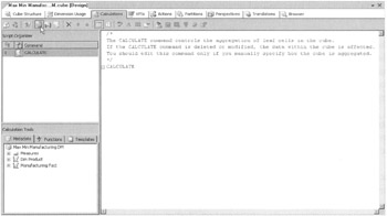
Figure 8-9: The Calculations tab

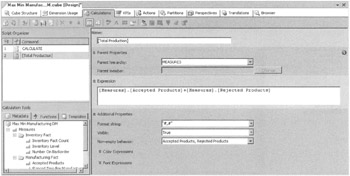
Figure 8-10: The Calculated Member form view

The name of the calculated measure is entered in Name. If the name contains one or more spaces, it must be enclosed in square brackets. Likewise, if the name contains one or more of the following characters:

 !@#$%^&*()-+=/?:;"'{ }\<>, 

it must be enclosed in square brackets.

Thus far, we have talked of calculated measures. However, it is possible to calculate members for dimensions as well. In fact, both calculated measures and calculated dimension members are referred to as calculated members, which is why the entry form is called the Calculated Member form. To specify that we are creating a calculated measure, MEASURES must be selected from the Parent Hierarchy drop-down list.

The actual definition of the calculated measure is entered in Expression. As mentioned earlier, this expression uses the MDX script language. The expression can be typed by hand or it can be built using the existing measures, MDX script functions, and templates found in the Calculation Tools window. This window can be seen in the lower-left of Figure 8-10.

The Format String drop-down list enables us to select the formatting to be applied to the calculation results. We can either select from one of the numeric formatting strings in the drop-down list or type in a custom format string. In most cases, one of the formatting strings from the drop-down list can do the job.

As we study MDX queries in Chapter 10, we learn about MDX queries that ask for only nonempty values from a measure. Rather than evaluating a calculated measure expression repeatedly to determine if it is nonempty, we can specify the conditions under which the calculation can produce a nonempty result. In most cases, this depends on whether one or more of the measures used in the calculation is nonempty.

The Non-empty Behavior drop-down list lets us select one or more measures in the cube. If any one of the selected measures is nonempty, the expression is executed to determine whether or not the resulting calculated measure is nonempty. When all of the selected measures are empty, the calculated measure is assumed to be empty without ever executing the expression.

In addition to the form view shown in Figure 8-10, we can also look at the underlying MDX script that completely defines the calculated measure. This is shown in Figure 8-11. Again, we explore the MDX script language more completely to understand this code in Chapter 10.

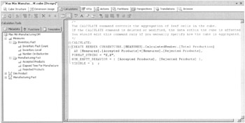
Figure 8-11: The Script view

We can use the measures in a cube in the expressions that define calculated measures in that cube. We can also use calculated measures in the expressions that define other calculated measures. This lets us break up complex calculations into much simpler building blocks that are easier to create and maintain.

It Doesn't Add Up—Measure Aggregates Other than SUM

We have already discussed how measures are aggregated along dimension hierarchies. By default, the Sum aggregate function is used for each measure. Measures that use the Sum function for their aggregation are additive measures.

In some cases, however, things just don't add up. In other words, there may be some measures that should not be summed along dimension hierarchies. For example, taking the sum of an average results in a number that is total nonsense. Instead, we always want to recalculate the average from the granular data. In other situations, we may want to use the maximum or minimum value for a measure along a dimension, rather than taking the sum. These measures are nonadditive measures.

The aggregate function used by a particular measure is controlled by the Aggregate property from that measure. Select the measure in the Measures window, and then use the Properties window to set the Aggregate property for this measure. This is shown in Figure 8-12.

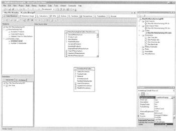
Figure 8-12: Setting the aggregate function for a measure

Semiadditive Measures

Certain measures may be added along some dimensions, but not along others. For example, the inventory level measure can be added along the product dimension. The sum of the inventory amounts for each product yields the total number of products in the warehouse. However, the sum of the first three months' inventory amounts does not give the inventory amount at the end of the first quarter. This is shown in Figure 8-13.

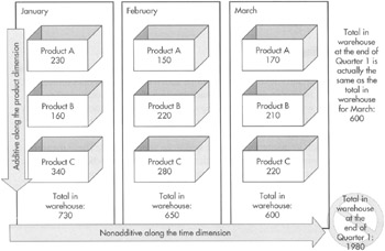
Figure 8-13: Inventory level is a semiadditive measure.

Measures such as inventory level are said to be semiadditive. These measures must use a semiadditive measure to achieve the proper results when aggregating. Measures that use a semiadditive aggregate function must be related to a time dimension.

Aggregate Functions

Analysis Services provides a number of aggregate functions for use with measures in an OLAP cube.

Function	Additivity	Result
AverageOfChildren	Semiadditive	The average of all nonempty child members.
ByAccount	Semiadditive	Uses the aggregate function specified by an account dimension in the cube. If the cube does not include an account dimension, this aggregate function works the same as the None aggregate function.
Count	Semiaddilive	A count of the number of child members.
DistinctCount	Nonadditive	A count of the number of unique child members.
FirstChild	Semiadditive	The value of the first child member.
FirstNonEmpty	Semiadditive	The value of the first nonempty child member.
LastChild	Semiadditive	The value of the last child member.
LastNonEmpty	Semiadditive	The value of the last nonempty child member.
Max	Semiadditive	The greatest value of all child members.
Min	Semiadditive	The least value of all child members.
None	Nonadditive	No aggregation is done.
Sum	Additive	The sum of all child members. This is the default aggregate function for a measure.

Learn by Doing—Working with Measures and Measure Groups

Features Highlighted

• Adding formatting to a measure

• Adding a measure group to a cube

• Setting the aggregation function for a measure

• Creating calculated measures

Business Need We have not yet completed the vice president of production's change request for inventory and backorder information in the Max Min Manufacturing DM cube. We added a table for this information into the data mart and we populated that table from the Order Processing database. We now need to add these measures to the cube in a new measure group.

Once the inventory level measure is added to the cube, we need to specify the correct aggregate function for this measure. As noted earlier, inventory level is not additive. The inventory level for a given period of time is not the sum of the inventory levels within the period. Instead, inventory level is Semiadditive. The inventory level for a given period of time is the inventory level at the end of that period.

In addition, the vice president of production has come up with another change. He would like to see not only the number of accepted products produced and the number of rejected products produced, but also the total number of products produced. This, of course, is the sum of the number of accepted products, plus the number of rejected products. He also wants to see the number of rejected products produced as a percentage of the total number of products produced. We can implement these requests using calculated measures.

Steps

1. Open the Business Intelligence Development Studio.

2. Open the MaxMinManufacturingDM project.

3. In the Solution Explorer window, double-click the entry for Max Min Manufacturing DM.cube to display the Cube Design tab, if it is not already visible.

4. Expand the Manufacturing Fact measure group in the Measures window.

5. Select the Accepted Products measure.

6. In the Properties window, select #,# from the Format String drop-down list.

7. Select the Rejected Products measure in the Measures window.

8. In the Properties window, select #,# from the Format String drop-down list.

9. Select the Elapsed Time For Manufacture measure in the Measures window.

10. In the Properties window, select #,# from the Format String drop-down list.

11. Right-click in the Measures window and select New Measure Group from the Context menu. The New Measure Group dialog box appears.

12. Select Inventory Fact from the Select a Table from the Data Source View list and click OK to exit the New Measure Group dialog box. The InventoryFact table is added to the cube and the Inventory Fact measure group appears in the Measures window.

    Note 

    A red, wavy line is under the entry for the Inventory Fact measure group in the Measures window. The reason for this error notification is because we have not related this new measure group to any dimensions. We take care of this in the next learn By Doing exercise titled "Relating Dimensions in the Max Min Manufacturing DM Cube."

13. Expand the Inventory Fact measure group in the Measures window.

14. Select the Inventory Level measure.

15. In the Properties window, select LastNonEmpty from the drop-down list for the AggregateFunction property. The LastNonEmpty aggregate function is now used when aggregating this measure.

16. In the Properties window, select #,# from the Format String drop-down list.

17. Select the Number On Backorder measure in the Measures window.

18. In the Properties window, select LastNonEmpty from the drop-down list for the AggregateFunction property.

19. In the Properties window, select #,# from the Format String drop-down list.

20. Right-click the Inventory Fact Count measure in the Measures window and select Delete from the Context menu. The Delete Objects dialog box appears.

21. Click OK to confirm the deletion. The Cube Design tab should appear similar to Figure 8-14.

    Note 

    A count of the number of members in the measure group is automatically created when a new measure group is created. In this case, a count of the number of inventory entries is not a helpful measure, so it can be deleted.

22. Select the Calculations tab of the Cube Design tab to create calculated measures.

23. Click the New Calculated Member button in the Calculations tab toolbar. The Calculated Member form view appears.

24. Enter [Total Products] for Name. Enter the following for Expression:

     [Accepted Products] + [Rejected Products] 

25. Select #,# from the Format String drop-down list.

26. Check the Accepted Products and Rejected Products measures in the Nonempty Behavior selection window and click OK.

27. Click the New Calculated Member button in the Calculations tab toolbar. The Calculated Member form returns to the default values.

28. Enter [Percent Rejected] For Name. Enter the following for Expression:

     [Rejected Products] / [Total Products] 

29. Select Percent from the Format String drop-down list.

30. Check the Accepted Products and Rejected Products measures in the Nonempty Behavior selection window and click OK.

31. Click the Save All button in the toolbar.

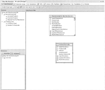
Figure 8-14: The Max Min Manufacturing DM cube with the Inventory Fact measure group