10.4. Dynamization for Worst-Case Performance

In the previous section, you saw that it is easy to amortize the cost of Insert and Delete analytically over time. The main idea for the construction of the dynamic data structure was given by the binary decomposition of W , which has fundamental changes from time to time, but the corresponding costs were amortized. Now, we are looking for the worst-case cost of Insert and Delete. The idea is to distribute the construction of V _j itself over time; i.e., the structure V _j should be finished if V _j _ˆ ₁ , V _j _ˆ ₂ , V has to be erased.

More precisely, we want to demonstrate that the given ideas can also be adapted for running under a cost model that measures every single operation in the worst case. The main ideas stem from [Overmars and van Leeuwen 81a, Overmars and van Leeuwen 81d].

For convenience, we consider the insert operation first. After a sequence of insert operations, we have to reconstruct the binary decomposition. Obviously, if this happens, the corresponding insert operation takes a lot of effort. Therefore, we will try to build up the new structure stepwise until the structure is already completed in the case of the last insertion.

The main idea is that every V _i is split into at most four structures: V _i ₁ , V _i ₂ , V _i ₃ , and V _i * with 2 ⁱ objects, respectively. V _i * is under construction. The general rule is as follows . If V _i ₁ is full and we insert objects into V _i ₂ for the first time, we start inserting the objects of V _i ₁ and V _i ₂ into V _i ₊₁ *, a structure of size 2 ⁱ ⁺¹ . This is spread over the next 2 ⁱ ⁺¹ insertions into V _i ₂ and V _i ₃ . Then, V _i ₊₁ * is full and replaces V _i _{+1 1} in the next insertion step. The second rule is that we successively replace , , or with V _i *, if V _i * is full. The replacement takes constant time.

For convenience, we consider a sequence of insertions into an empty structure. The steps can be seen in Figure 10.11.

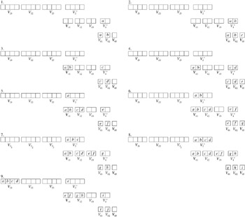
Figure 10.11: Spreading reconstruction over time.

The first object a is inserted into V ₀₁ . The next object b is inserted into V ₀₂ . At the same time, application of the simple rule above requires that the first element of V ₀₁ = a is inserted into V ₁ *.
c is inserted into V ₀₃ . At the same time, V ₀₂ = b is inserted into V ₁ ^* , and V ₁ * is finished for the first time. That is, we successively build up V ₁ * from the elements of V ₀₁ and V ₀₂ after two insertions.
If the next element d has to be inserted, V ₀₁ , V ₀₂ , and V ₀₃ are already full. Now, V ₁₁ is replaced by V ₁ ^* and V ₀₁ is replaced by V ₀₃ , and the new element d is inserted into V ₀₃ . This again means that we start to build a new V ₁ * with elements of V ₀₁ and V ₀₂ , and c is inserted into V ₁ *.
The next element e is inserted into V ₀₃ , and at the same time, d is inserted into V ₁ *, which is completed then.
If the next element f is inserted, V ₁₂ is replaced by V ₁ *. With respect to the above rule, the first part of V ₂ * is constructed with the first element of V ₁₁ , which is a .
The element g is inserted into V ₀₃ , V ₁ * is completed, and V ₂ * has half-size.
V ₁ * replaces V ₁₃ , if h is inserted. Again, we start with a new construction of V ₁ * by inserting V ₀₁ = g .
If i is inserted into V ₀₃ , the structure V ₂ * is completed after the 2 ² insertions, namely of f , g , h , and i . Again, V ₁ * is completed also.
In the next step, V ₂ * replaces V ₂₁ . Additionally, V ₁₃ replaces V ₁₁ and V ₁ * is moved to V ₁₂ . Therefore, we also start to build up V ₁ * again from V ₁₁ and V ₁₂ .

The structure V _i ₊₁ * is completed after 2 ⁱ ⁺¹ insert operations. Altogether, for every single insert operation, we invest

time for the construction of V _i ₊₁ *. Of course, we still need to sum up the cost for all structures V _i *. The cost can be analyzed analogously to the amortized cost in Section 10.3.1. The only difference to the amortized cost model is that the work has to be partially done if the insert operations occurs.

The structures V _i ₁ , V _i ₂ and V _i ₃ are either full or empty. For the query operation, all full structures V _i ₁ , V _i ₂ , and V _i ₃ are in use.

We have to take care that the Build and Collect operations can be split into small steps; otherwise , we cannot distribute the work adequately.

A worst-casesensitive delete operation for the binary decomposition can be implemented as follows. We start to reconstruct a better copy V of each of the single structures V if the number of all (real data and weakly deleted elements) objects n in V equals approximately 3/2 times the number of the real data objects in V . If the number of all (real data and weakly deleted elements) objects n of V rise to approximately two times the number of the real data objects, V should should be ready to replace V .

The structures V _i ₁ , V _i ₂ , and V _i ₃ may have weakly deleted elements. For a single WeakDelete, we will find the corresponding substructure by a balanced search tree, as shown in the previous section. As explained earlier, we start to reconstruct V _ij in a copy if 1/4 of the structure V _ij is non-real . If the half-size of the structure V _ij becomes non-real, we replace V _ij by . We have to take care that is fully completed if the half-size limit is reached. The worst case is that after the start of constructing , only WeakDelete operations occur. In any case, at least 1/4 V _ij WeakDelete operations can be used to build . Therefore, the cost b _V ( V _ij ) is spread over 1/4 V _ij WeakDelete operations, and each operation is charged with cost

The main difference from the amortized cost model is that the work has to be partially done if the WeakDelete operation occurs.

There is one special problem here. Some of the real objects of V _ij that were already inserted in the copy may be weakly deleted before is ready. During the reconstruction of V _ij in , we cannot perform a WeakDelete on the copy . Therefore, we store the WeakDelete operations on V _ij in a queue and apply them afterwards to . Thus, if V _ij is replaced by , it may have some weakly deleted objects. But it can be guaranteed by simple arithmetic that less than 25 per cent of the new structure is non-real. There is also a special problem with V _i *. We cannot weakly delete elements from , because we still have to construct it. Therefore, for V _i *, we also store the WeakDelete operations on and in a queue and apply them afterwards to V _i *.

We refer the interested reader to [Klein 05] and [Overmars 83] for more information.

Theorem 10.5. A static abstract data type Static , as presented in Figure 10.10 with an additional operation V . WeakDelete( d ) and with additional cost function wd _V ( n ) , can be dynamized in a dynamic abstract data type DYNAMIC so that

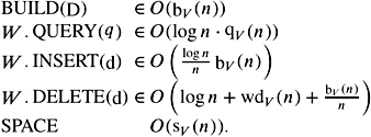
Here, n denotes the number actual data objects.