Coding of Still Pictures (JPEG and JPEG2000)
Overview
In the mid 1980s joint work by the members of the ITU-T (International Telecommunication Union) and the ISO (International Standards Organisation) led to standardisation for the compression of grey scale and colour still images [1]. This effort was then known as JPEG: the Joint Photographic Experts Group. As is apparent, the word joint refers to the collaboration between the ITU-T and ISO. The JPEG encoder is capable of coding full colour images at an average compression ratio of 15:1 for subjectively transparent quality [2]. Its design meets special constraints, which make the standard very flexible. For example, the JPEG encoder is parametrisable, so that the desired compression/quality trade-offs can be determined based on the application or the wishes of the user [3].
JPEG can also be used in coding of video, on the basis that video is a succession of still images. In this case the process is called motion JPEG. Currently, motion JPEG has found numerous applications, the most notable one being video coding for transmission over packet networks with unspecified bandwidth or bit rates (UBR). A good example of UBR networks is the Internet where, due to unpredictability of the network load, congestion may last for a significant amount of time. Since in motion JPEG each frame is independently coded, it is an ideal encoder of video for such a hostile environment.
Another application of motion JPEG is video compression for recording on magnetic tapes, where again the independent coding of pictures increases the flexibility of the encoder for recording requirements, such as editing, pause, fast forward, fast rewind etc. Also, such an encoder can be very resilient to loss of information, since the channel error will not propagate through the image sequence. However, since the coding of I-pictures in the MPEG-2 standard is similar to motion JPEG, normally video compression for recording purposes is carried out with the I-picture part of the MPEG-2 encoder. The I-pictures are those which are encoded without reference to previous or subsequent pictures. This will be explained in Chapter 7.
At the turn of the millennium, the JPEG committee decided to develop another standard for compression of still images, named the JPEG2000 standard [4]. This was in response to growing demands for multimedia, Internet and a variety of digital imagery applications. However, in terms of compression methodology these two standards are very different. Hence in order to discriminate between them, throughout the book, the original JPEG is called JPEG and the new one JPEG2000.
Lossless compression
The JPEG standard specifies two classes of encoding and decoding, namely lossless and lossy compression. Lossless compression is based on a simple predictive DPCM method using neighbouring pixel values, and DCT is employed for the lossy mode.
Figure 5.1 shows the main elements of a lossless JPEG image encoder.
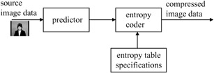
Figure 5.1: Lossless encoder
The digitised source image data in the form of either RGB or YCbCr is fed to the predictor. The image can take any format from 4:4:4 down to 4:1:0, with any size and amplitude precision (e.g. 8 bits/pixel). The predictor is of the simple DPCM type (see Figure 3.1), where every individual pixel of each colour component is differentially encoded. The prediction for an input pixel x is made from combinations of up to three neighbouring pixels at positions a, b and c from the same picture of the same colour component, as shown in Figure 5.2.
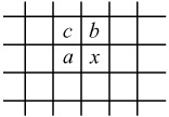
Figure 5.2: Three-sample prediction neighbourhood
The prediction is then subtracted from the actual value of the pixel at position x, and the difference is losslessly entropy coded by either Huffman or arithmetic coding. The entropy table specifications unit determines the characteristics of the variable length codes of either entropy coding method.
The encoding process might be slightly modified by reducing the precision of input image samples by one or more bits prior to lossless coding. For lossless processes, sample precision is specified to be between 2 and 16 bits. This achieves higher compression than normal lossless coding, but has lower compression than DCT-based lossy coding for the same bit rate and image quality. Note that this is in fact a type of lossy compression, since reduction in the precision of input pixels by b bits is equivalent to the quantisation of the difference samples by a quantiser step size of 2b.
Lossy compression
In addition to lossless compression, the JPEG standard defines three lossy compression modes. These are called the baseline sequential mode, the progressive mode and the hierarchical mode. These modes are all based on the discrete cosine transform (DCT) to achieve a substantial compression while producing a reconstructed image with high visual fidelity. The main difference between these modes is the way in which the DCT coefficients are transmitted.
The simplest DCT-based coding is referred to as the baseline sequential process and it provides capability that is sufficient for many applications. The other DCT-based processes which extend the baseline sequential process to a broader range of applications are referred to as extended DCT-based processes. In any extended DCT-based decoding processes, baseline decoding is required to be present in order to provide a default decoding capability.
Baseline sequential mode compression
Baseline sequential mode compression is usually called baseline coding for short. In this mode, an image is partitioned into 8 × 8 nonoverlapping pixel blocks from left to right and top to bottom. Each block is DCT coded, and all the 64 transform coefficients are quantised to the desired quality. The quantised coefficients are immediately entropy coded and output as part of the compressed image data, thereby minimising coefficient storage requirements.
Figure 5.3 illustrates the JPEG's baseline compression algorithm. Each eight-bit sample is level shifted by subtracting 28-1=7 = 128 before being DCT coded. This is known as DC level shifting. The 64 DCT coefficients are then uniformly quantised according to the step size given in the application-specific quantisation matrix. The use of a quantisation matrix allows different weighting to be applied according to the sensitivity of the human visual system to a coefficient of the frequency.
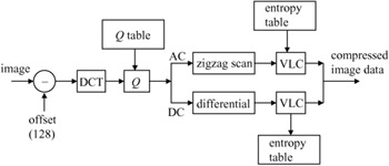
Figure 5.3: Block diagram of a baseline JPEG encoder
Two examples of quantisation tables are given in Tables 5.1 and 5.2. [5]. These tables are based on psychovisual thresholding and are derived empirically using luminance and chrominance with a 2:1 horizontal subsampling. These tables may not be suitable for any particular application, but they give good results for most images with eight-bit precision.
|
16 |
11 |
10 |
16 |
24 |
40 |
51 |
61 |
|
12 |
12 |
14 |
19 |
26 |
58 |
60 |
55 |
|
14 |
13 |
16 |
24 |
40 |
57 |
69 |
56 |
|
14 |
17 |
22 |
29 |
51 |
87 |
80 |
62 |
|
18 |
22 |
37 |
56 |
68 |
109 |
103 |
77 |
|
24 |
35 |
55 |
64 |
81 |
104 |
113 |
92 |
|
49 |
64 |
78 |
87 |
103 |
121 |
120 |
101 |
|
72 |
92 |
95 |
98 |
112 |
100 |
103 |
99 |
If the elements of the quantisation tables of luminance and chrominance are represented by Q(u, v), then a quantised DCT coefficient with horizontal and vertical spatial frequencies of u and v, Fq(u, v), is given by:
| (5.1) | 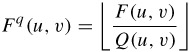 |
|
17 |
18 |
24 |
47 |
99 |
99 |
99 |
99 |
|
18 |
21 |
26 |
66 |
99 |
99 |
99 |
99 |
|
24 |
26 |
56 |
99 |
99 |
99 |
99 |
99 |
|
47 |
66 |
99 |
99 |
99 |
99 |
99 |
99 |
|
99 |
99 |
99 |
99 |
99 |
99 |
99 |
99 |
|
99 |
99 |
99 |
99 |
99 |
99 |
99 |
99 |
|
99 |
99 |
99 |
99 |
99 |
99 |
99 |
99 |
|
99 |
99 |
99 |
99 |
99 |
99 |
99 |
99 |
where F(u, v) is the transform coefficient value prior to quantisation, and ⌊.⌋ means rounding the division to the nearest integer. At the decoder the quantised coefficients are inverse quantised by:
| (5.2) |  |
to reconstruct the quantised coefficients.
A quality factor q_JPEG is normally used to control the elements of the quantisation matrix Q(u, v) [6]. The range of q_JPEG percentage values is between 1 and 100 per cent. The JPEG quantisation matrices of Tables 5.1 and 5.2 are used for q_JPEG = 50, for the luminance and chrominance, respectively. For other quality factors, the elements of the quantisation matrix, Q(u, v), are multiplied by the compression factor a, defined as [6]:
| (5.3) | 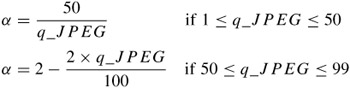 |
subject to the condition that the minimum value of the modified quantisation matrix elements, αQ(u, v), is 1. For 100 per cent quality, q_JPEG = 100, that is lossless compression; all the elements of αQ(u, v) are set to 1.
After quantisation, the DC (commonly referred to as (0,0)) coefficient and the 63 AC coefficients are coded separately as shown in Figure 5.3. The DC coefficients are DPCM coded with prediction of the DC coefficient from the previous block, as shown in Figure 5.4, i.e. DIFF = DCi - DCi-1. This separate treatment from the AC coefficients is to exploit the correlation between the DC values of adjacent blocks and to code them more efficiently as they typically contain the largest portion of the image energy. The 63 AC coefficients starting from coefficient AC(1,0) are run length coded following a zigzag scan as shown in Figure 5.4.
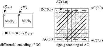
Figure 5.4: Preparing of the DCT coefficients for entropy coding
The adoption of a zigzag scanning pattern is to facilitate entropy coding by encountering the most likely nonzero coefficients first. This is due to the fact that, for most natural scenes, the image energy is mainly concentrated in a few low frequency transform coefficients.
Run length coding
Entropy coding of the baseline encoder is accomplished in two stages. The first stage is the translation of the quantised DCT coefficients into an intermediate set of symbols. In the second stage, variable length codes are assigned to each symbol. For the JPEG standard a symbol is structured in two parts: a variable length code (VLC) for the first part, normally referred to as symbol-1, followed by a binary representation of the amplitude for the second part, symbol-2.
5.2.2.1 Coding of DC coefficients
Instead of assigning individual variable length codewords (e.g. Huffman code) to each DIFF, the DIFF values are categorised based on the magnitude range called CAT. The CAT is then variable length coded. Table 5.3 shows the categories for the range of amplitudes in the baseline JPEG. Since the DCT coefficient values are in the range -2047 to 2047, there are 11 categories for nonzero coefficients. Category zero is not used for symbols; it is used for defining the end of block (EOB) code.
|
CAT |
Range |
|---|---|
|
0 |
- |
|
1 |
-1, 1 |
|
2 |
-3, -2, 2,3 |
|
3 |
-7,...-4, 4,...7 |
|
4 |
-15, ...-8, 8, ...15 |
|
5 |
-31, ...-16, 16,...31 |
|
6 |
-63, ...-32, 32, ...63 |
|
7 |
-127, ... -64, 64, ... 127 |
|
8 |
-255, ...-128, 128, ...255 |
|
9 |
-511,... -256, 256, ...511 |
|
10 |
-1023, ...-512, 512, ...1023 |
|
11 |
-2047,... -1024, 1024,... 2047 |
The CAT after being VLC coded is appended with additional bits to specify the actual DIFF values (amplitude) within the category. Here CAT is symbol-1 and the appended bits represent symbol-2.
When the DIFF is positive the appended bits are just the lower order bits of the DIFF. When it is negative, the appended bits become the lower order bits of DIFF-1. The lower order bits start from the point where the most significant bit of the appended bit sequence is one for positive differences and zero for negative differences. For example: for DIFF = 6 = 0000 ... 00110, the appended bits start from 1, hence it would be 110. This is because DIFF is positive and the most significant bit of the appended bits should be 1. Also, since 6 is in the range of 4 to 7 (Table 5.3) the value of CAT is 3. From Table B.1 of Appendix B, the codeword for CAT = 3 is 100. Thus the overall codeword for DIFF = 6 is 100110, where 100 is the VLC code of CAT (symbol-1) and 110 is the appended codeword (symbol-2).
For a negative DIFF, such as DIFF = -3, first of all -3 is in the range of -3 to -2, thus from Table 5.3, CAT = 2, and its VLC code from Table B.1 of Appendix B is 011. However, to find the appended bits, DIFF - 1 = -4 = 1111 ... 100, where the lower order bits are 00. Note the most significant bit of the appended bits is 0. Thus the codeword becomes 01100.
5.2.2.2 Coding of AC coefficients
For each nonzero AC coefficient in zigzag scan order, symbol-1 is described as a two-dimensional event of (RUN, CAT), sometimes called (RUN, SIZE). For the baseline encoder, CAT is the category for the amplitude of a nonzero coefficient in the zigzag order, and RUN is the number of zeros preceding this nonzero coefficient. The maximum length of run is limited to 15. Encoding of runs greater than 15 is done by a special symbol (15, 0), which is a run length of 15 zero coefficients followed by a coefficient of zero amplitude. Hence it can be interpreted as the extension symbol with 16 zero coefficients. There can be up to three consecutive (15, 0) symbols before the terminating symbol-1 followed by a single symbol-2. For example a (RUN = 34, CAT = 5) pair would result in three symbols a, b, and c, with a = (15, 0), b = (15, 0) and c = (2, 5).
An end of block (EOB) is designated to indicate that the rest of the coefficients of the block in the zigzag scanning order are quantised to zero. The EOB symbol is represented by (RUN = 0, CAT = 0).
The AC code table for symbol-1 consists of one Huffman codeword (maximum length 16 bits, not including additional bits) for each possible composite event. Table B.2 of Appendix B shows the codewords for all possible combinations of RUN and CAT of symbol-1 [4]. The format of the additional bits (symbol-2) is the same as in the coding of DIFF in DC coefficients. For the kth AC coefficient in the zigzag scan order, ZZ(k), the additional bits are either the lower order bits of ZZ(k) when ZZ(k) is positive, or the lower order bits of ZZ(k) - 1, when ZZ(k) is negative. In order to clarify this, let us look at a simple example.
Example: the quantised DCT coefficients of a luminance block are shown in Figure 5.5. If the DC coefficient in the previous luminance block was 29, find the codewords for coding of the DC and AC coefficients.
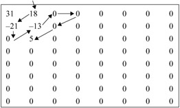
Figure 5.5: Quantised DCT coefficients of a luminance block
Codeword for the DC coefficient
DIFF = 31 - 29 = 2. From Table 5.3, CAT = 2 and according to Table B.1 of Appendix B, the Huffman code for this value of CAT is 011. To find the appended bits, since DIFF = 2 > 0, then 2 = 000 ... 0010. Thus the appended bits are 10. Hence the overall codeword for coding the DC coefficient is 01110.
Codewords for the AC coefficients
Scanning starts from the first nonzero AC coefficient that has a value of 18. From Table 5.3, the CAT value for 18 is 5, and since there is no zero value AC coefficient before it, then RUN = 0. Hence, symbol-1 is (0, 5). From Table B.2 of Appendix B, the codeword for (0, 5) is 11010. The symbol-2 is the lower order bits of ZZ(k) = 18 = 000 ... 010010, which is 10010. Thus the first AC codeword is 1101010010.
The next nonzero AC coefficient in the zigzag scan order is -21. Since it has no zero coefficient before it and it is in the range of -31 to -16, then it has a RUN = 0, and CAT = 5. Thus symbol-1 of this coefficient is (0, 5), which again from Table B.2 of Appendix B, has a codeword of 11010. For symbol-2, since -21 < 0, then ZZ(k) - 1 = -21 - 1 = -22 = 111... 1101010, and symbol-2 becomes 01010 (note the appended bits start from where the most significant bit is 0). Thus the overall codeword for the second nonzero AC coefficient is 1101001010.
The third nonzero AC coefficient in the scan is -13, which has one zero coefficient before it. Then RUN = 1 and, from its range, CAT is 4. From Table B.2 of Appendix B, the codeword for (RUN = 1, CAT = 4) is 111110110. To find symbol-2, ZZ(k) -1 = -13 - 1 = -14 = 111... 110010. Thus symbol-2 = 0010, and the whole codeword becomes 1111101100010.
The fourth and the final nonzero AC coefficient is 5 (CAT = 3), which is preceded by three zeros (RUN = 3). Thus symbol-1 is (3, 3), which, from Table B.2 of Appendix B, has a codeword of 111111110101. For symbol-2, since ZZ(k) = 5 = 000 ... 00101, then the lower order bits are 101, and the whole codeword becomes 111111110101101.
Since 5 is the last nonzero AC coefficient, then the encoding terminates here and the end of block (EOB) code is transmitted which is defined as the (0, 0) symbol with no appended bits. From Table B.2 of Appendix B, its codeword is 1010.
5.2.2.3 Entropy coding
For coding of the magnitude categories or run length events, the JPEG standard specifies two alternative entropy coding methods, namely Huffman coding and arithmetic coding. Huffman coding procedures use Huffman tables, and the type of table is determined by the entropy table specifications, shown in Figure 5.3. Arithmetic coding methods use arithmetic coding conditioning tables, which may also be determined by the entropy table specification. There can be up to four different Huffman and arithmetic coding tables for each DC and AC coefficient. No default values for Huffman tables are specified, so the applications may choose tables appropriate for their own environment. Default tables are defined for the arithmetic coding conditioning. Baseline sequential coding uses Huffman coding, and extended DCT-based and lossless processes may use either Huffman or arithmetic coding (see Table 5.4).
|
Baseline process (required for all DCT-based decoders)
|
|
Extended DCT-based processes
|
|
Lossless process
|
|
Hierarchical processes
|
In arithmetic coding of AC coefficients, the length of zero run is no longer limited to 15; it can go up to the end of the block (e.g. 62). Also, arithmetic coding may be made adaptive to increase the coding efficiency. Adaptive means that the probability estimates for each context are developed based on a prior coding decision for that context. The adaptive binary arithmetic coder may use a statistical model to improve encoding efficiency. The statistical model defines the contexts which are used to select the conditional probability estimates used in the encoding and decoding procedures.
Extended DCT based process
The baseline encoder only supports basic coding tools, which are sufficient for most image compression applications. These include input image with eight-bit/pixel precision, Huffman coding of the run length, and sequential transmission. If other modes, or any input image precision, are required, and in particular if arithmetic coding is employed to achieve higher compression, then the term extended DCT-based process is applied to the encoder. Table 5.4 summarises all the JPEG supported coding modes.
Figure 5.6 illustrates the reconstruction of a decoded image in a sequential mode (baseline or extended). As mentioned, as soon as a block of pixels is coded, its 64 coefficients are quantised, coded and transmitted. The receiver after decoding the coefficients, inverse quantisation and inverse transformation, sequentially adds them to the reconstructed image. Depending on the channel rate, it might take some time to reconstruct the whole image. In Figure 5.6, reconstructed images at 25, 50, 75 and 100 per cent of the image are shown.
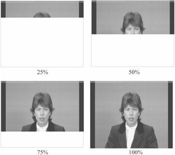
Figure 5.6: Reconstructed images in sequential mode
In the progressive mode, the quantised coefficients are stored in the local buffer and transmitted later. There are two procedures by which the quantised coefficients in the buffer may be partially encoded within a scan. Firstly, for the highest image quality (lowest quantisation step size) only a specified band of coefficients from the zigzag scanned sequence need to be coded. This procedure is called spectral selection, since each band typically contains coefficients which occupy a lower or higher part of the frequency spectrum for the 8 × 8 block. Secondly, the coefficients within the current band need not be encoded to their full accuracy within each scan (coarser quantisation). On a coefficient's first encoding, a specified number of the most significant bits are encoded first. In subsequent scans, the less significant bits are then encoded. This procedure is called successive approximation or bit plane encoding. Either procedure may be used separately, or they may be mixed in flexible combinations.
Figure 5.7 shows the reconstructed image quality with the first method. In this Figure, the first image is reconstructed from the DC coefficient only, with its full quantised precision. The second image is made up of DC (coefficient 0) plus the AC coefficients 1 and 8, according to the zigzag scan order. That is, after receiving the two new AC coefficients, a new image is reconstructed from these coefficients and the previously received DC coefficients. The third image is made up of coefficients 0, 1, 8, 16, 9, 2, 3, 10, 17 and 24. In the last image, all the significant coefficients (up to EOB) are included.
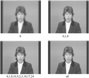
Figure 5.7: Image reconstruction in progressive mode
Hierarchical mode
In the hierarchical mode, an image is coded as a sequence of layers in a pyramid. Each lower size image provides prediction for the next upper layer. Except for the top level of the pyramid, for each luminance and colour component at the lower levels the difference between the source components and the reference reconstructed image is coded. The coding of the differences may be done using only DCT-based processes, only lossless processes, or DCT-based processes with a final lossless process for each component.
Downsampling and upsampling filters, similar to those of Figures 2.4 and 2.6, may be used to provide a pyramid of spatial resolution, as shown in Figure 5.8. The hierarchical coder including the downsampling and upsampling filters is shown in Figure 5.9.
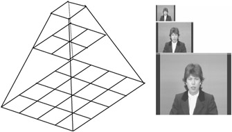
Figure 5.8: Hierarchical multiresolution encoding
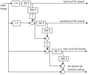
Figure 5.9: A three-level hierarchical encoder
In this Figure, the image is lowpass filtered and subsampled by 4:1, in both directions, to give a reduced image size 1/16. The baseline encoder then encodes the reduced image. The decoded image at the receiver may be interpolated by 1:4 to give the full size image for display. At the encoder, another baseline encoder encodes the difference between the subsampled input image by 2:1 and the 1:2 upsampled decoded image. By repeating this process, the image is progressively coded, and at the decoder it is progressively built up. The bit rate at each level depends on the quantisation step size at that level. Finally, for lossless reversibility of the coded image, the difference between the input image and the latest decoded image is lossless entropy coded (no quantisation).
As we see, the hierarchical mode offers a progressive representation similar to the progressive DCT-based mode, but it is useful in environments which have multiresolution requirements. The hierarchical mode also offers the capability of progressive transmission to a final lossless stage, as shown in Figure 5.9.
Extra features
In coding of colour pictures, encoding is called noninterleaved if all blocks of a colour component are coded before beginning to code the next component. Encoding is interleaved if the encoder compresses a block of 8 × 8 pixels from each component in turn, considering the image format. For example, with the 4:4:4 format, one block from each luminance and two chrominance components are coded. In the 4:2:0 format, the encoder codes four luminance blocks before coding one block from each of Cb and Cr.
The encoder is also flexible to allow different blocks within a single component to be compressed using different quantisation tables resulting in a variation in the reconstructed image quality, based on their perceived relative importance. This method of coding is called region of interest (ROI) coding. Also, the standard can allow different regions within a single image block to be compressed at different rates.
JPEG2000
Before describing the basic principles of the JPEG2000 standard, it might be useful to understand why we need another standard. Perhaps the most convincing explanation is that, since the introduction of JPEG in the 1980s, too much has changed in the digital image industry. For example, current demands for compressed still images range from web logos of sizes less than 10 Kbytes to high quality scanned images of the order of 5 Gbytes!! [8]. The existing JPEG surely is not optimised to efficiently code such a wide range of images. Moreover, scalability and interoperability requirements of digital imagery in a heterogeneous network of ATM, Internet, mobile etc., make the matter much more complicated.
The JPEG2000 standard is devised with the aim of providing the best quality or performance and capabilities to market evolution that the current JPEG standard fails to cater for. In the mean time it is assumed that Internet, colour facsimile, printing, scanning, digital photography, remote sensing, mobile, medical imagery, digital libraries/archives and e-commerce are among the most immediate demands. Each application area imposes a requirement that JPEG2000 should fulfil. Some of the most important features [9] that this standard aims to deliver are:
Superior low bit rate performance: this standard should offer performance superior to the current standards at low bit rates (e.g. below 0.25 bit per pixel for highly detailed greyscale images). This significantly improved low bit rate performance should be achieved without sacrificing performance on the rest of the rate distortion spectrum. Examples of applications that need this feature include image transmission over networks and remote sensing. This is the highest priority feature.
Continuous tone and bilevel compression: it is desired to have a standard coding system that is capable of compressing both continuous tone and bilevel images [7]. If feasible, the standard should strive to achieve this with similar system resources. The system should compress and decompress images with various dynamic ranges (e.g. 1 bit to 16 bit) for each colour component. Examples of applications that can use this feature include compound documents with images and text, medical images with annotation overlays, graphic and computer generated images with binary and near-to-binary regions, alpha and transparency planes, and facsimile.
Lossless and lossy compression: it is desired to provide lossless compression naturally in the course of progressive decoding (i.e. difference image encoding, or any other technique, which allows for the lossless reconstruction to be valid). Examples of applications that can use this feature include medical images where loss is not always tolerable, image archival pictures where the highest quality is vital for preservation but not necessary for display, network systems that supply devices with different capabilities and resources, and prepress imagery.
Progressive transmission by pixel accuracy and resolution: progressive transmission that allows images to be reconstructed with increasing pixel accuracy or spatial resolution is essential for many applications. This feature allows the reconstruction of images with different resolutions and pixel accuracy, as needed or desired, for different target devices. Examples of applications include web browsing, image archiving and printing.
Region of interest coding: often there are parts of an image that are more important than others. This feature allows a user-defined region of interest (ROI) in the image to be randomly accessed and/or decompressed with less distortion than the rest of the image.
Robustness to bit errors: it is desirable to consider robustness to bit errors while designing the code stream. One application where this is important is wireless communication channels. Portions of the code stream may be more important than others in determining decoded image quality. Proper design of the code stream can aid subsequent error correction systems in alleviating catastrophic decoding failures. Use of error confinement, error concealment, restart capabilities, or source channel coding schemes can help minimise the effects of bit errors.
Open architecture: it is desirable to allow open architecture to optimise the system for different image types and applications. With this feature, the decoder is only required to implement the core tool set and a parser that understands the code stream. If necessary, unknown tools are requested by the decoder and sent from the source.
Protective image security: protection of a digital image can be achieved by means of methods such as: watermarking, labelling, stamping, fingerprinting, encryption, scrambling etc. Watermarking and fingerprinting are invisible marks set inside the image content to pass a protection message to the user. Labelling is already implemented in some imaging formats such as SPIFF, and must be easy to transfer back and forth to the JPEG2000 image file. Stamping is a mark set on top of a displayed image that can only be removed by a specific process. Encryption and scrambling can be applied on the whole image file or limited to part of it (header, directory, image data) to avoid unauthorised use of the image.
JPEG2000 encoder
The JPEG2000 standard follows the generic structure of the intraframe still image coding introduced for the baseline JPEG. That is, decorrelating the pixels within a frame by means of transformation and then quantising and entropy coding of the quantised transform coefficients for further compression. However, in order to meet the design requirements set forth in section 5.3, in addition to the specific requirements from the transformation and coding, certain preprocessing on the pixels and post processing of the compressed data is necessary. Figure 5.10 shows a block diagram of a JPEG2000 encoder.
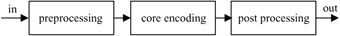
Figure 5.10: A general block diagram of the JPEG2000 encoder
In presenting this coder, we only talk about the fundamentals behind this standard. More details can be found in the ISO standardisation documents and several key papers [9–11].
Preprocessor
Image pixels prior to compression are preprocessed to make certain goals easier to achieve. There are three elements in this preprocessor.
5.4.1.1 Tiling
Partitioning the image into rectangular nonoverlapping pixel blocks, known as tiling, is the first stage in preprocessing. The tile size is arbitrary and can be as large as the whole image size down to a single pixel. A tile is the basic unit of coding, where all the encoding operations, from transformation down to bit stream formation, are applied to tiles independent of each other. Tiling is particularly important for reducing memory requirement and, since they are coded independently, any part of the image can be accessed and processed differently from the other parts of the image. However, due to tiling, the correlation between the pixels in adjacent tiles is not exploited, and hence as the tile size is reduced, the compression gain of the encoder is also reduced.
5.4.1.2 DC level shifting
Similar to DC level shifting in the JPEG standard (Figure 5.3), values of the RGB colour components within the tiles are DC shifted by 2B-1, for B bits per colour component. Such an offset makes certain processing, such as numerical overflow, arithmetic coding, context specification etc. simpler. In particular, this allows the lowest subband, which is a DC signal, to be encoded along with the rest of the AC wavelet coefficients. At the decoder, the offset is added back to the colour component values.
5.4.1.3 Colour transformation
There are significant correlations between the RGB colour components. Hence, prior to compression by the core encoder, they are decorrelated by some form of transformation. In JPEG2000 two types of colour decorrelation transform are recommended.
In the first type, the decorrelated colour components Y, Cb and Cr, are derived from the three colour primaries R, G and B according to:
| (5.4) |  |
Note that this transformation is slightly different from the one used for coding colour video (see section 2.2). Also note that since transformation matrix elements are approximated (not exact), then even if YCbCr are losslessly coded, the decoded RGB colour components cannot be free from loss. Hence this type of colour transformation is irreversible, and it is called irreversible colour transformation (ICT). ICT is used only for lossy compression.
The JPEG2000 standard also defines a colour transformation for lossless compression. Therefore, the transformation matrix elements are required to be integer. In this mode, the transformed colour components are referred to as Y, U and V, and are defined as:
| (5.5) | 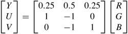 |
Here the colour decorrelation is not as good as ICT, but it has the property that if YUV are losslessly coded, then exact values of the original RGB can be retrieved. This type of transformation is called reversible colour transformation (RCT). RCT may also be used for lossy coding, but since ICT has a better decorrelation property than RCT, use of RCT can reduce the overall compression efficiency.
It is worth mentioning that in compression of colour images, colour fidelity may be traded for that of luminance. In the JPEG standard this is done by subsampling the chrominance components Cb and Cr, or U and V, like the 4:2:2 and 4:2:0 image formats. In JPEG2000, image format is always 4:4:4, and the colour subsampling is done by the wavelet transform of the core encoder. For example, in coding of a 4:4:4 image format, if the highest LH, HL and HH bands of Cb and Cr chrominance components are set to zero, it has the same effect as coding of a 4:2:0 image format.
Core encoder
Each transformed colour component of YCbCr/YUV is coded by the core encoder. As in the JPEG encoder, the main elements of the core encoder are: transformation, quantisation and entropy coding. Thus a more detailed block diagram of JPEG2000 is given by Figure 5.11.
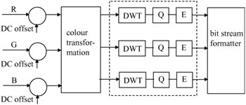
Figure 5.11: The encoding elements of JPEG2000
In the following sections these elements and their roles in image compression are presented.
5.4.2.1 Discrete wavelet transform
In JPEG2000, transformation of pixels that in the JPEG standard used DCT has been replaced by the discrete wavelet transform (DWT). This has been chosen to fulfil some of the requirements set forth by the JPEG2000 committee. For example:
- Multiresolution image representation is an inherent property of the wavelet transform. This also provides simple SNR and spatial scalability, without sacrificing compression efficiency.
- Since the wavelet transform is a class of lapped orthogonal transforms then, even for small tile sizes, it does not create blocking artefacts.
- For larger dimension images, the number of subband decomposition levels can be increased. Hence, by exploiting a larger area of pixel intercorrelation a higher compression gain can be achieved. Thus for images coded at low bit rates, DWT is expected to produce better compression gain than the DCT which only exploits correction with 8 × 8 pixels.
- DWT with integer coefficients, such as the (5,3) tap wavelet filters, can be used for lossless coding. Note that in DCT, since the cosine elements of the transformation matrix are approximated, lossless coding is not then possible.
The JPEG2000 standard recommends two types of filter bank for lossy and lossless coding. The default irreversible transform used in the lossy compression is the Daubechies 9-tap/7-tap filter [12]. For the reversible transform, with a requirement for lossless compression, it is LeGall and Tabatabai's 5-tap/3-tap filters as they have integer coefficients [13]. Table 5.5 shows the normalised coefficients (rounded to six decimal points) of the lowpass and highpass analysis filters H0(z)/H1(z) of the 9/7 and 5/3 filters. Those of the synthesis G0 (z) and G1(z) filters can be derived from the usual method of G0(z) = H1 (-z) and G1 (z) = -H0(-z).
|
Coefficients |
Lossy compression (9/7) |
Lossless compression (5/3) |
||
|---|---|---|---|---|
|
lowpass H0(z) |
highpass H1(z) |
lowpass H0(z) |
highpass H1(z) |
|
|
0 |
+0.602949 |
+1.115087 |
3/4 |
1 |
|
±1 |
+0.266864 |
-0.591272 |
1/4 |
-1/2 |
|
±2 |
-0.078223 |
-0.057544 |
-1/8 |
|
|
±3 |
-0.016864 |
+0.091272 |
||
|
±4 |
+0.026729 |
|||
Note that to preserve image energy in the pixel and wavelet domains, the integer filter coefficients in lossless compression are normalised for unity gain. Since the lowpass and highpass filter lengths are not equal, these types of filter are called biorthogonal. The lossy 9/7 Daubechies filter pairs [12] are also biorthogonal.
5.4.2.2 Quantisation
After the wavelet transform, all the coefficients are quantised linearly with a dead band zone quantiser (Figure 3.5). The quantiser step size can vary from band to band and since image tiles are coded independently, it can also vary from tile to tile. However, one quantiser step size is allowed per subband of each tile. The choice of the quantiser step size can be driven by the perceptual importance of that band on the human visual system (HVS), similar to the quantisation weighting matrix used in JPEG (Table 5.1), or by other considerations, such as the bit rate budget.
As mentioned in Chapter 4, wavelet coefficients are most efficiently coded when they are quantised by successive approximation, which is the bit plane representation of the quantised coefficients. In this context the quantiser step size in each subband, called the basic quantiser step size, A, is related to the dynamic range of that subband, such that the initial quantiser step size, after several passes, ends up with the basic quantiser step size A. In JPEG2000, the basic quantiser step size for band b, Δb, is represented with a total of two bytes, an 11-bit mantissa μb and a five-bit exponent εb according to the relationship:
| (5.6) | 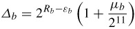 |
where Rb is the number of bits representing the nominal dynamic range of subband b. That is  is greater than the magnitude of the largest coefficient in subband b. Values of μb and εb for each subband are explicitly transmitted to the decoder. For lossless coding, used with reversible (5,3) filter banks, μb = 0 and εb = Rb, which results in Δb = 1. On the other hand, the maximum value of Δb is almost twice the dynamic range of the input sample when εb = 0 and μb has its maximum value, which is sufficient for all practical cases of interest.
5.4.2.3 Entropy coding
The indices of the quantised coefficients in each subband are entropy coded to create the compressed bit stream. In Chapter 4 we introduced three efficient methods of coding these indices, namely: EZW, SPIHT and EBCOT. As mentioned in section 4.7, the JPEG committee chose embedded block coding with optimised truncation (EBCOT), due to its many interesting features that fulfil the JPEG2000 objectives. Details of EBCOT were given in section 4.7, and here we only summarise its principles and show how it is used in the JPEG2000 standard.
In EBCOT, each subband of an image tile is partitioned into small rectangular blocks, called code blocks, and code blocks are encoded independently. The dimensions of the code blocks are specified by the encoder and, although they may be chosen freely, there are some constraints; they must be an integer power of two; the total number of coefficients in a code block cannot exceed 4096 and the height of the code block cannot be less than four. Thus the maximum length of the code block is 1024 coefficients.
The quantiser indices of the wavelet coefficients are bit plane encoded one bit at a time, starting from the most significant bit (MSB) and preceding to the least significant bit (LSB). During this progressive bit plane encoding, if the quantiser index is still zero, that coefficient is called insignificant. Once the first nonzero bit is encoded, the coefficient becomes significant and its sign is encoded. For significant coefficients, all subsequent bits are referred to as refinement bits. Since in the wavelet decomposition the main image energy is concentrated at lower frequency bands, many quantiser indices of the higher frequency bands will be insignificant at the earlier bit planes. Clustering of insignificant coefficients in bit planes creates strong redundancies among the neighbouring coefficients that are exploited by JPEG2000 through a context-based adaptive arithmetic coding.
In JPEG2000, instead of encoding the entire bit plane in one pass, each bit plane is encoded in three subbit plane passes. This is called fractional bit plane encoding, and the passes are known as: significance propagation pass, refinement pass and clean up pass. The reason for this is to be able to truncate the bit stream at the end of each pass to create the near optimum bit stream. Here, the pass that results in the largest reduction in distortion for the smallest increase in bit rate is encoded first.
In the significance propagation pass, the bit of a coefficient in a given bit plane is encoded if and only if, prior to this pass, the coefficient was insignificant and at least one of its eight immediate neighbours was significant. The bit of the coefficient in that bit plane, 0 or 1, is then arithmetically coded with a probability model derived from the context of its eight immediate neighbours. Since neighbouring coefficients are correlated, it is more likely that the coded coefficient becomes significant, resulting in a large reduction in the coding distortion. Hence this pass is the first to be executed in fractional bit plane coding.
In the refinement pass, a coefficient is coded if it was significant in the previous bit plane. Refining the magnitude of a coefficient reduces the distortion moderately. Finally, those coefficients that were not coded in the two previous passes are coded in the clean up pass. These are mainly insignificant coefficients (having eight insignificant immediate neighbours) and are likely to remain insignificant. Hence their contribution in reducing distortions is minimal and is used in the last pass. For more details of coding, refer to EBCOT in section 4.7.
Postprocessing
Once the entire image has been compressed, the bit stream generated by the individual code blocks is postprocessed to facilitate various functionalities of the JPEG2000 standard. This part is similar to the layer formation and bit stream organisation of EBCOT known as tier 2 (see section 4.7).
To form the final bit stream, the bits generated by the three spatially consistent coded blocks (one from each subband at each resolution level) comprise a packet partition location, called a precinct [10]. A collection of packets, one from each precinct, at each resolution level comprises the layer. Figure 5.12 shows the relationship between the packetised bit stream and the units of image, such as the code block, precinct, tile and the image itself.
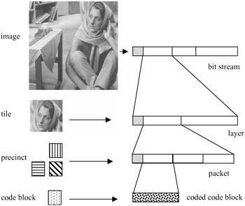
Figure 5.12: Correspondence between the spatial data and bit stream
Here, the smallest unit of compressed data is the coded bits from a code block. Data from three code blocks of a precinct makes a packet, with an appropriate header, addressing the precinct position in the image. Packets are then grouped into the layer and finally form the bit stream, all with their relevant headers to facilitate flexible decoding. Since precincts correspond to spatial locations, a packet could be interpreted as one quality increment for one resolution at one spatial location. Similarly, a layer could be viewed as one quality increment for the entire image. Each layer successively and gradually improves the image quality and resolution, so that the decoder is able to decode the code block contributions contained in the layer, in sequence. Since ordering of packets into the layer and hence into the bit stream can be as desired, various forms of progressive image transmission can be realised.
Some interesting features of JPEG2000
Independent coding of code blocks and flexible multiplexing of quality packets into the bit stream exhibit some interesting phenomena. Some of the most remarkable features of JPEG2000 are outlined in the following.
Region of interest
In certain applications, it might be desired to code parts of a picture at a higher quality than the other parts. For example, in web browsing one might be interested in a logo of a complex web page image that needs to be seen first. This part needs to be given higher priority for transmission. Another example is in medical images, where the region of interest (ROI) might be an abnormality in the part of the whole image that requires special attention.
Figure 5.13 shows an example of a ROI, where the head and scarf of Barbara are coded at a higher quality than the rest of the picture, called the background. Loss of image quality outside the region of interest (outside the white box), in particular on the tablecloth, trousers and the books, is very clear.
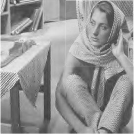
Figure 5.13: Region of interest with better quality
Coding of the region of interest in the JPEG2000 standard is implemented through the so-called maxshift method [14]. The basic principle in this method is to scale (shift) up the coefficients, such that their bits are placed at a higher level than the bits associated with the background data, as shown in Figure 5.14. Depending on the scale value, S, some bits of the ROI coefficients might be encoded together with those of the background, like Figure 5.14a, or all the bits of the ROI are encoded before any background data are coded, as shown in Figure 5.14b. In any case, the ROI at the decoder is decoded or refined before the rest of the image.
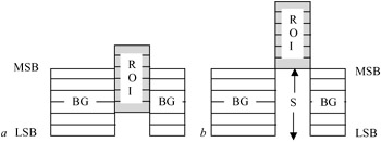
Figure 5.14: Scaling of the ROI coefficients
It is interesting to note that, if the value of scaling S is computed such that the minimum coefficient belonging to the ROI is larger than the maximum coefficient of the background, then it is possible to have arbitrary shaped ROIs, without the need for defining the ROI shape to the decoder. This is because every received coefficient that is smaller than S belongs to the background, and can be easily identified.
Scalability
Scalability is one of the important parts of all the image/video coding standards. Scalable image coding means being able to decode more than one quality or resolution image from the bit stream. This allows the decoders of various capabilities to decode images according to their processing powers or needs. For example, although low performance decoders may decode only a small portion of the bit stream, providing basic quality or resolution images, high performance decoders may decode a larger portion of the bit stream, proving higher quality images. The most well known types of scalability in JPEG2000 are the SNR and spatial scalabilities. Since in JPEG2000, code blocks are individually coded, bit stream scalability is easily realised. In order to have either SNR or spatial scalability, the compressed data from the code blocks should be inserted into the bit stream in the proper order.
Spatial scalability
In spatial scalability, from a single bit stream, images of various spatial resolutions can be decoded. The smaller size picture with an acceptable resolution is the base layer and the parts of the bit stream added to the base layer to create higher resolution images comprise the next enhancement layer, as shown in Figure 5.15.
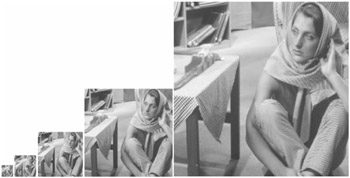
Figure 5.15: Spatial scalable decoding
In JPEG2000, due to the octave band decomposition of the wavelet transform, spatial scalability is easily realised. In this mode, compressed data of the code blocks has to be packed into the bit stream such that all the bit planes of the lower level subbands precede those of the higher bands.
SNR scalability
The signal-to-noise ratio (SNR) scalability involves producing at least two levels of image of the same spatial resolutions, but at different quality, from a single bit stream. The lowest quality image is called the base layer, and the parts of the bit stream that enhance the image quality are called enhancement layers. In JPEG2000, through bit plane encoding, the lowest significant bit plane that gives an acceptable image quality can be regarded as the base layer image. Added quality from the subsequent bit planes produces a set of enhanced images. Figure 5.16 shows a nine-layer SNR scalable image produced by bit plane coding from a single layer, where the compressed code block data from a bit plane of all the subbands is packed before the data from the next bit plane.
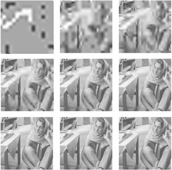
Figure 5.16: SNR scalable decoding
In Figure 5.16 the first picture is made up from coding the most significant bit of the lowest LL band. As bit plane coding progresses towards lower bits, more bands are coded, improving the image quality. Any of the images can be regarded as the base layer, but for an acceptable quality, picture number four or five may just meet
the criterion. The remaining higher quality images become its enhanced versions at different quality levels.
Resilience
Compressed bit streams, especially those using variable length codes (e.g. arithmetic coding) are extremely sensitive to channel errors. Even a single bit error may destroy the structure of the following valid codewords, corrupting a very large part of the image. Resilience and robustness to channel errors are the most desired features expected from any image/video encoder. Fortunately in JPEG2000, since the individual quality packets can be independently decoded, the effect of channel errors can be confined to the area covered by these packets. This is not the case with the other wavelet transform encoders such as EZW and SPIHT. Figure 5.17 shows the impact of a single bit error on the reconstructed picture, encoded by the SPIHT and JPEG2000. As the Figure shows, although a single bit error destroys the whole picture encoded by SPIHT, its effect on JPEG2000 is only limited to a small area, around Barbara's elbow. It is worth noting that the SPIHT encoder, even without arithmetic coding, is very sensitive to channel errors. For example, a single bit error in the early pass of LIS (refer to section 4.6) can corrupt the whole image, as can be seen from Figure 5.17a. In fact, this picture is not arithmetically coded at all, and the single bit error was introduced at the first pass of the LIS data. Of course it is possible to guard EZW and SPIHT compressed data against channel errors. For instance, if the bit stream generated by each tree of EZW/SPIHT can be marked, then propagation of errors into the trees can be prevented. This requires some extra bits to be inserted between the tree's bit streams as resynchronisation markers. This inevitably increases the bit rate. Since the resynchronisation marker bits are fixed in rate, irrespective of the encoded bit rate, the increase in bit rate is more significant at lower bit rates than at higher bit rates. For example, in coding Barbara with SPIHT at 0.1, 0.5 and 1 bit/pixel, the overhead in bits will be 2.7, 0.64 and 0.35 per cent, respectively.
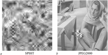
Figure 5.17: Effect of single bit error on the reconstructed image, encoded by SPIHT and JPEG2000
Problems
|
1. |
The luminance quantisation Table 5.1 is used in the baseline JPEG for a quality factor of 50 per cent. Find the quantisation table for the following quality factors:
|
|
||||||||||||||||||||||||||||||||||||||||||||||||||||||||||||||||
|
2. |
In problem 1 find the corresponding tables for the chrominance. |
|
||||||||||||||||||||||||||||||||||||||||||||||||||||||||||||||||
|
3. |
The DCT transform coefficients (luminance) of an 8 x 8 pixel block prior to quantisation are given by:
Find the quantisation indices for the baseline JPEG with the quality factors of:
|
|
||||||||||||||||||||||||||||||||||||||||||||||||||||||||||||||||
|
4. |
In problem 3, if the quantised index of the DC coefficient in the previous block was 50, find the pairs of symbol-1 and symbol-2 for the given quality factors. |
|
||||||||||||||||||||||||||||||||||||||||||||||||||||||||||||||||
|
5. |
Derive the Huffman code for the 25 per cent quality factor of problem 4 and hence calculate the number of bits required to code this block. |
|
||||||||||||||||||||||||||||||||||||||||||||||||||||||||||||||||
|
6. |
A part of the stripe of the wavelet coefficients of a band is given as:
Assume the highest bit plane is 6. Using EBCOT identify which coefficient is coded at bit plane 6 and which one at bit plane 5. In each case identify the type of fractional bit plane used. |
|

Answers
|
1. |
|
||||||||||||||||||||||||||||||||||||||||||||||||||||||||||||||||||||||||||||||||||||||||||||||||||||||||||||||||||||||||||||||||
|
2. |
the same as problem 1. |
||||||||||||||||||||||||||||||||||||||||||||||||||||||||||||||||||||||||||||||||||||||||||||||||||||||||||||||||||||||||||||||||
|
3. |
|
||||||||||||||||||||||||||||||||||||||||||||||||||||||||||||||||||||||||||||||||||||||||||||||||||||||||||||||||||||||||||||||||
|
4. |
for 50% quality: DIFF = 62 - 50 = 12, symbol_1 = 4; symbol_2 = 12 scanned pairs (3,1)(0,3)(0,1)(0,-1)(1,-1)(6,1)(6,1)(1,1)(1,1)(35,3) and the resultant events: (3,1)(0,2)(0,1)(0,1)(1,1)(6,1)(6,1)(1,1)(1,1)(15,0)(15,0)(3,3) for 25% quality: DIFF= 31-50 = -19, symbol_1 = 5, symbol_2 = -19-1 =-20 scanned pairs: (4, 1)(57, 1) events: (4,1)(15,0)(15,0)(15,0)(9,1) |
||||||||||||||||||||||||||||||||||||||||||||||||||||||||||||||||||||||||||||||||||||||||||||||||||||||||||||||||||||||||||||||||
|
5. |
for DC: DIFF= -19 ⇒ CAT = 5; DIFF-1 = -20 VLC for CAT = 5 is 110 and -20 in binary is 11101100, hence the VLC for the DC coefficient is 11001100 for AC, using the AC VLC tables: for each (15,0) the VLC is 11111111001 and for (9, 1) the VLC is 111111001 total number of bits: 8 + 3 x 11 + 9 = 50 bits. |
||||||||||||||||||||||||||||||||||||||||||||||||||||||||||||||||||||||||||||||||||||||||||||||||||||||||||||||||||||||||||||||||
|
6. |
At bit-plane 6 coefficient 65 at clean-up pass. At bit-plane 5 coefficient 65 at all passes and coefficient 50 at clean-up pass. |
 , and small elements of the matrix will be 1 and larger ones become 2.
References
1 ISO 10918-1 (JPEG): 'Digital compression and coding of continuous-tone still images'. 1991
2 FURHT, B.: 'A survey of multimedia compression techniques and standards. Part I: JPEG standard', Real-Time Imaging, 1995, pp. 1–49
3 WALLACE, G.K.: 'The JPEG still picture compression standard', Commun. ACM, 1991, 34:4, pp.30–44
4 JPEG2000: 'JPEG2000 part 2, final committee draft'. ISO/IEC JTC1/SC29/WG1 N2000, December 2000
5 PENNEBAKER, W.B., and MITCHELL, J.L.: 'JPEG: still image compression standard' (Van Nostrand Reinhold, New York, 1993)
6 The independent JPEG Group: 'The sixth public release of the Independent JPEG Group's free JPEG software'. C source code of JPEG encoder release 6b, March 1998, [ftp://ftp.uu.net/graphics/jpeg/jpegsrc_v6b_tar.gz]
7 WANG, Q., and GHANBARI, M.: 'Graphics segmentation based coding of multimedia images', Electron. Lett., 1995, 31:6, pp.542–544
8 SKODRAS, A.,CHRISTOPOULOS, C., and EBRAHIMI, T.: 'The JPEG2000 still image compression standard', IEEE Signal Process. Mag., September 2001, pp.36–58
9 'Visual evaluation of JPEG-2000 colour image compression performance'. ISO/IECJTC1/SC29/WG1 N1583, March 2000
10 RBBANI, M., and JOSHI, R.: 'An overview of the JPEG2000 image compression standard', Signal Process. Image Commun., 17:1, January 2002, pp.3–48
11 SANTA-CRUZ, D.,GROSBOIS, R., and EBRAHIMI, T.: 'JPEG2000 performance evaluation and assessment', Signal Process., Image Commun. 17:1, January 2002, pp.
12 DAUBECHIES, I.: 'The wavelet transform, time frequency localization and signal analysis, IEEE Trans Inf. Theory, 1990, 36:5, pp.961–1005
13 LE GALL, D., and TABATABAI, A.: 'Subband coding of images using symmetric short kernel filters and arithmetic coding techniques'. IEEE international conference on Acoustics, speech and signal processing, ICASSP'88, 1988, pp.761–764
14 CHRISTOPOULOS, C.A.,ASKELF, J., and LARSSON, M.: 'Efficient methods for encoding regions of interest in the up-coming JPEG2000 still image coding standard', IEEE Signal Process. Lett., 2000, 7, pp.247–249
Page not found. Sorry. :(
EAN: 2147483647
Pages: 148
