5. Shot Segmentation

5. Shot Segmentation

Because shot segmentation is a prerequisite for virtually any task involving the understanding, parsing, indexing, characterization, or categorization of video, the grouping of video frames into shots has been an active topic of research in the area of multimedia signal processing. Extensive evaluation of various approaches has shown that simple thresholding of histogram distances performs surprisingly well and is difficult to beat [18].

5.1 Bayesian Shot Segmentation

We have developed an alternative formulation that regards the problem as one of statistical inference between two hypotheses:

• H₀: no shot boundary occurs between the two frames under analysis (S = 0),

• H₁: a shot boundary occurs between the two frames (S = 1),

for which the minimum probability of error decision is achieved by a likelihood ratio test [19] where H₁ is chosen if

(3.1)

and H₀ is chosen otherwise. It can easily be verified that thresholding is a particular case of this formulation, in which both conditional densities are assumed to be Gaussian with equal covariance. From the discussion in the previous section, it is clear that this does not hold for real video. One further limitation of the thresholding model is that it does not take into account the fact that the likelihood of a new shot transition is dependent on how much time has elapsed since the previous one.

We have, however, shown in [13] that the statistical formulation can be extended to overcome these limitations, by taking into account the shot duration models of section 3. For this, one needs to consider the posterior odds ratio between the two hypotheses

(3.2)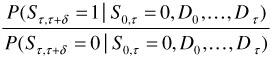

where S_a,b is the state of interval [a, b], δ is the duration of each frame (inverse of frame rate), and D_τ is the activity measurement at time τ. Under the assumption of stationarity for D_τ, and a generic Markov property (D_τ independent of all previous D and S given S_τ,_τ+δ), it is possible to show that the optimal decision (in the minimum probability of error sense) is to declare that a boundary exists in [τ,τ+δ] if

(3.3)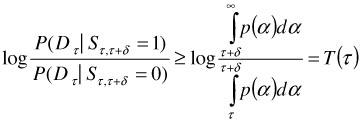

and that there is no boundary otherwise. Comparing this with (1), it is clear that the inclusion of the shot duration prior transforms the fixed threshold approach into an adaptive one, where the threshold depends on how much time has elapsed since the previous shot boundary.

It is possible to derive closed-form expressions for the optimal threshold for both the Erlang and Weibull priors [13], namely

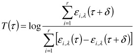
for the former and

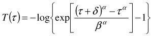
for the latter. The evolution of the thresholds over time for both cases is presented in Figure 3.4. While in the initial segment of the shot the threshold is large and shot changes are unlikely to be accepted, the threshold decreases as the scene progresses increasing the likelihood that shot boundaries will be declared. The intuitive nature of this procedure is a trademark of Bayesian inference [20] where, once the mathematical details are worked out, one typically ends up with a solution that is intuitively correct.

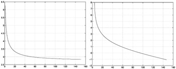
Figure 3.4: Temporal evolution of the Bayesian threshold for the Erlang (left) and Weibull (right) priors ( 2000 IEEE).

While qualitatively similar, the two thresholds exhibit important differences in terms of their steady state behaviour. Ideally, in addition to decreasing monotonically over time, the threshold should not be lower bounded by a positive value as this may lead to situations in which its steady-state value is large enough to miss several consecutive shot boundaries. While the Erlang prior fails to meet this requirement (due to the constant arrival rate assumption discussed in section 3), the Weibull prior does lead to a threshold that decreases to -∞ as τ grows. This guarantees that a new shot boundary will always be found if one waits long enough. In any case, both the Erlang and Weibull priors lead to adaptive thresholds that are more intuitive than the fixed threshold in common use for shot segmentation.

5.2 Shot Segmentation Results

The performance of Bayesian shot segmentation was evaluated on a database containing the promotional trailers of Figure 3.1. Each trailer consists of 2 to 5 minutes of video and the total number of shots in the database is 1959. In all experiments, performance was evaluated by the leave-one-out method. Ground truth was obtained by manual segmentation of all the trailers.

We evaluated the performance of Bayesian models with Erlang, Weibull, and Poisson shot duration priors and compared them against the best possible performance achievable with a fixed threshold. For the latter, the optimal threshold was obtained by brute-force, i.e., testing several values and selecting the one that performed best. The total number of errors, misses (boundaries that were not detected), and false positives (regular frames declared as boundaries) achieved with all priors are shown in Figure 3.5. It is visible that, while the Poisson prior leads to worse accuracy than the static threshold, both the Erlang and the Weibull priors lead to significant improvements. The Weibull prior achieves the overall best performance decreasing the error rate of the static threshold by 20%. A significantly more detailed analysis of the relative performance of the various priors can be found in [13].

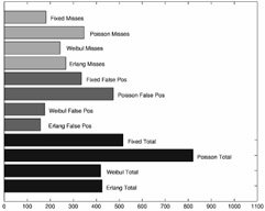
Figure 3.5: Total number of errors, false positives, and missed boundaries achieved with the different shot duration priors ( 2000 IEEE).

The reasons for the improved performance of Bayesian segmentation are illustrated in Figure 3.6, which presents the evolution of the thresholding process for a segment from one of the trailers in the database ("blankman"). Two approaches are depicted: Bayesian with the Weibull prior, and standard fixed thresholding. The adaptive behaviour of the Bayesian threshold significantly increases the robustness against spurious peaks of the activity metric originated by events such as very fast motion, explosions, camera flashes, etc. This is visible, for example, in the shot between frames 772 and 794 which depicts a scene composed of fast moving black and white graphics where figure and ground are frequently reversed. While the Bayesian procedure originates a single false-positive, the fixed threshold produces several. This is despite the fact that we have complemented the plain fixed threshold with commonly used heuristics, such as rejecting sequences of consecutive shot boundaries [18]. The vanilla fixed threshold would originate many more errors.

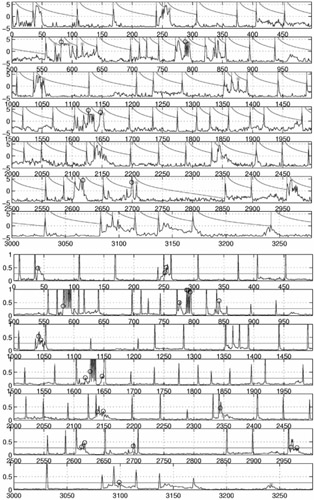
Figure 3.6: Evolution of the thresholding operation for a challenging trailer. Top— Bayesian segmentation. The likelihood ratio and the Weibull threshold are shown. Bottom— Fixed threshold. The histogram distances and the optimal threshold are presented. In both graphs, misses are represented as circles and false positives as stars ( 2000 IEEE).