4. Data Reorganization

4. Data Reorganization

An important goal for any computer cluster is to achieve a balanced load distribution across all the nodes. Both round-robin and random data placement techniques, described in Sec. 2, distribute data retrievals evenly across all disk drives over time. A new challenge arises when additional nodes are added to a server in order to a) increase the overall storage capacity of the system, or b) increase the aggregate disk bandwidth to support more concurrent streams. If the existing data are not redistributed then the system evolves into a partitioned server where each retrieval request will impose a load on only part of the cluster. One might try to even out the load by storing new media files on only the added nodes (or at least skewed towards these nodes), but because future client retrieval patterns are usually not precisely known this solution becomes ineffective.

Redistributing the data across all the disks (new and old) will once again yield a balanced load on all nodes. Reorganizing blocks placed in a random manner requires much less overhead when compared to redistributing blocks placed using a constrained placement technique. For example, with round-robin striping, when adding or removing a disk, almost all the data blocks need to be relocated. More precisely, z_j blocks will move to the old and new disks and B-z_j blocks will stay put as defined in Eq. 1:

(1)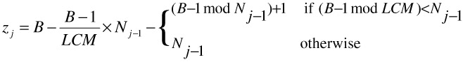

where B is the total number of object blocks, N_j is the number of disks upon the j^th scaling operation and LCM is the least common multiple of N_j-1 and N_j. Instead, with a randomized placement, only a fraction of all data blocks need to be moved. To illustrate, increasing a storage system from four to five disks requires that only 20% of the data from each disk be moved to the new disk. Assuming a well-performing pseudo-random number generator, z_j blocks move to the newly added disk(s) and B-z_j blocks stay on their disks where z_j is approximated as:

(2)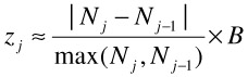

z_j is approximated since it is the theoretical percentage of block moves. z_j should be observed when using a 32-bit pseudo-random number generator and the number of disks and blocks increases. The number of block moves is simulated in Figure 32.3a as disks are scaled one-by-one from 1 to 200. Similarly for disk removal, only the data blocks on the disk that are scheduled for removal must be relocated. Redistribution with random placement must ensure that data blocks are still randomly placed after disk scaling (adding or removing disks) to preserve the load balance.

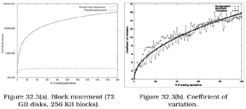
Figure 32.3: Block movement and coefficient of variation.

As described in Sec. 2, we use a pseudo-random number generator to place data blocks across all the disks of Yima. Each data block is assigned a random number, X, where X mod N is the disk location and N is the number of disks. If the number of disks does not change, then we are able to reproduce the random location of each block. However, upon disk scaling, the number of disks changes and some blocks need to be moved to different disks in order to maintain a balanced load. Blocks that are now on different disks cannot be located using the previous random number sequence; instead a new random sequence must be derived from the previous one.

In Yima we use a composition of random functions to determine this new sequence. Our approach, termed SCAling Disks for Data Arranged Randomly (SCADDAR), preserves the pseudo-random properties of the sequence and results in minimal block movements after disk scaling while it computes the new locations for data blocks with little overhead [11]. This algorithm can support scaling of disks while Yima is online through either an eager or lazy method; the eager method uses a separate process to move blocks while the lazy method moves blocks as they are accessed.

We call the new random numbers, which accurately reflect the new block locations after disk scaling, X_j, where j is the scaling operation (j is 0 for the initial random numbers generated by the pseudo-random number generator). We wish to map X₀ to X_j for every block at every scaling operation, j, such that X_j mod N_j results in the new block locations. We have formulated Eqs. 3 and 4 to compute the new X_j's for an addition of disks and a removal of disks, respectively:

(3)

(4)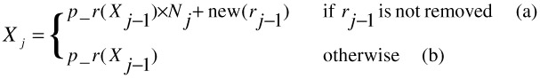

In order to find X_j (and ultimately the block location at X_j mod N_j) we must first compute X₀, X₁, X₂, …, X_j-1. Eqs. 3 and 4 compute X_j by using X_j-1 as the seed to the pseudo-random number generator so we can ensure that X_j and X_j-1 are independent. We base this on the assumption that the pseudo-random function performs well.

We can achieve our goal of a load balanced storage system where similar loads are imposed on all the disks on two conditions: uniform distribution of blocks and random placement of these blocks. A uniform distribution of blocks on disks means that all disks contain the same (or similar) number of blocks. So, we need a metric to show that SCADDAR achieves a balanced load. We would like to use the uniformity of the distribution as a metric; hence, the standard deviation of the number of blocks across disks is a suitable choice. However, because the averages of blocks per disk will differ when scaling disks, we normalize the standard deviation and use the coefficient of variation (standard deviation divided by average) instead. One may argue that a uniform distribution may not necessarily result in a random distribution since, given 100 blocks, the first 10 blocks may reside on the first disk, the second 10 blocks may reside on the second disk, and so on. However, given a perfect pseudo-random number generator (one that outputs independent X_j's that are all uniformly distributed between 0 and R), SCADDAR is statistically indistinguishable from complete reorganization. ^[5] This fact can be easily proven by demonstrating a coupling between the two schemes; due to lack of space, we omit the proofs from this chapter version. However, since real life pseudo-random number generators are unlikely to be perfect, we cannot formally analyze the properties of SCADDAR so we use simulation to compare it with complete reorganization instead. Thus, SCADDAR does result in a satisfactory random distribution. For the rest of this section, we use the uniformity of block distribution as an indication of load balancing.

We performed 100 disk scaling operations with 4000 data blocks. Figure 32.3b shows the coefficient of variations of three methods when scaling from 1 to 100 disks (one-by-one). The first curve shows complete block reorganization after adding each disk. Although complete reorganization requires a great amount of block movement, the uniform distribution of blocks is ideal. The second curve shows SCADDAR. This follows the trend of the first curve suggesting that the uniform distribution is maintained at a near-ideal level while minimizing block movement. The third curve shows the theoretical coefficient of variation as defined in Def. 32.1. The theoretical coefficient of variation is derived from the theoretical standard deviation of Bernoulli trials. The SCADDAR curve also follows a similar trend as the theoretical curve.

(Definition 32.1) Theoretical coefficient of variation is a percentage and defined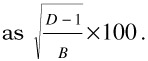

When adding disks to a disk array, the average disk bandwidth usage across the array will decrease after data are redistributed using SCADDAR. The resulting load balanced placement leads to more available bandwidth which can be used to support additional streams. We measure the bandwidth usage of a disk within a disk array as the array is scaled. In Figure 32.4a, we show the disk bandwidth of one disk among the array when the array size is scaled from 2 to 7 disks (1 disk added every 120 seconds beginning at 130 seconds). 10 clients are each receiving 5.33 Mbps streams across the duration of the scaling operations. The bandwidth continues to decrease and follows the expected bandwidth (shown as the solid horizontal lines) as the disks are scaled. While the bandwidth usage of each disk decreases, we observe in Figure 32.4b that the total bandwidth of all disks remains fairly level and follows the expected total bandwidth (53.3 Mbps); fluctuations are due to the variable bitrate of the media.

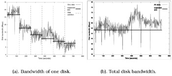
Figure 32.4: Disk bandwidth when scaling from 2 to 7 disks. One disk is added every 120 seconds (10 clients each receiving 5.33 Mbps).

^[5]This does not mean that SCADDAR and complete reorganization will always give identical results; the two processes are identical in distribution.