3. The Video Algebra

3. The Video Algebra

Having defined a video formally, we are now ready to define the video algebra. The video algebra consists of extensions of extensions of relational algebra operations (like select, project, Cartesian product, join, union, intersection, and difference). In the rest of this section, we define these operations one by one. Our first operation is selection.

3.1 Selection

Our approach to defining selection consists of three major parts. The first part involves specifying the syntax of a selection condition. The second part involves specifying when a block sequence satisfies a given selection condition. Once these two parts are defined, it is a simple matter to say that the result of applying a selection (using selection condition C) to a video v consists of those block sequences in v that satisfy selection condition C. It is important to note that we will be reasoning about block sequences rather than individual blocks. This is necessary because some conditions in a video may need to be evaluated not over a single block, but over a block sequence.

3.1.1 Selection Conditions: Syntax

Throughout this paper, we assume the existence of some arbitrary, but fixed set VP of visual predicates. A visual predicate takes a visual object or activity as input (perhaps with other nonvisual inputs as well) and evaluates to either true or false. Examples of visual predicates include:

• color(rect1,rect2,dist,d): This predicate succeeds if the color histograms of two rectangles (sub-images of an image) are within distance dist of each other when using a distance metric d.

• texture(rect1,rect2,dist,d): This predicate succeeds if the texture histograms of two rectangles (sub-images of an image) are within distance dist of each other when using a distance metric d.

• shape(rect1,rect2,dist,d): This predicate succeeds if the shapes of two rectangles are within a distance dist of each other when using distance metric d.

It is important to note that the above three visual predicates can actually be implemented in many different ways. Section 3.1.3 gives several examples of how to implement these visual predicates using, for instance, color histograms, wavelets for implementing texture distances and wavelet-based shape descriptors.

As our algebra can work with any visual predicates whatsoever, we continue with the algebraic treatment here, and leave the example visual predicate descriptions of Section 3.1.4. We start with the concept of a path.

Definition (path) Suppose o is an object.

• If o's type is in {int,real,string} then ε_real, ε_int, ε_string are all paths for o of types int,real,string, respectively. When clear from context, we will just write ε (without the subscript).

• If o's type is [A₁ : τ₁,…,A_n : τ_n] and p_i is a path for an object of type τ, then A_i p_i is a path for o whose type is the type of p_i.

• If o's type is {τ}, and p is a path for objects of type τ, then p is a path for o also with the same type τ.

Intuitively, paths are used to access the interior components of a complex type. For example, if we have an attribute called color of type [red:int,green:int,blue:int] and we want to find all very "bluish" objects, we may use the path expression color.blue to reference the blue component of the color attribute of an object.

We are now ready to define selection conditions.

Definition (selection condition) Suppose T is a set of types VP, p₁ and p₂ are paths over the same type τ ∈ T, v ∈ d om(τ), and VP is a set of visual predicates. Then:

1. p₁ θ p₂, and p₁ θ v, and vθ p₂ are selection conditions. Here, θ is one of the following:

   • If τ is a domain with an associated partial ordering ≤, then θ∈ {=,≥,≤,>,<}.

   • Otherwise θ is the equality symbol "="'.

2. Every visual predicate is a selection condition.

3. If C₁, C₂ are selection conditions and k ≥ 0 is an integer, then so are (C₁ ∧ C₂), (C₁ ∨ C₂), before(k, C₁), after(k, C₁).

Example. Here are some simple selection conditions.

• O.color.blue > 200 is satisfied by objects whose "blue" field has a value over 200.

• O1.color.blue > O2.color.blue is satisfied by pairs of objects, with the first one more "blue" than the other one.

• O1.color.blue > O2.color.red is satisfied by pairs of objects such that the blue component of the first object is greater than the red component of the second one.

• O.color.blue > 200 AND O.color.red <20 AND O.color.green < 20 may be used in our stork example to find water (as this is quite blue and the red and green components are very small).

• Color(rect1,rect2,10,L1) is a visual predicate which succeeds if rectangle rect1 is within 10 units of distance of rectangle rect2 using a distance metric called L1. In section 3.1.2, we do introduce one such distance metric.

It is important to note that visual predicates are satisfied by regions, while path conditions such as those in item (1) of the definition of a selection condition are satisfied by objects.

3.1.2 Selection Conditions: Semantics

We are now ready to define the semantics of selection conditions. Suppose v is a video and ρ is its association map. Throughout this paper, we assume that there is some oracle O that can automatically check if a visual predicate is true or not.

In practice, this oracle is nothing more than the code that implements the visual predicates (e.g., the various matching algorithms). We now define what it means for a block sequence to satisfy a selection condition.

Definition (satisfaction) Suppose O is an oracle that evaluates visual predicates, b is a block and C is a selection condition. We say that b satisfies C w.r.t. O, denoted b ⊨ C, iff:

1. C is a visual predicate and O(C)= true.

2. C is of the form (pθv) and there exists o ∈ ρ(b), o.p is well defined and (o.p = v') and (v' θ v) holds.

3. C is of the form (p₁ θ p₂), there exist o₁,o₂ ∈ ρ(b), not necessarily distinct, o₁.p₁ and o₂.p₂ are well defined, (o₁.p₁ = v'), (o₂.p₂ =v"), and (v' θv") holds.

4. C is of the form (C₁ ∧ C₂) and b ⊨ C₁ and b ⊨ C₂

5. C is of the form (C₁ ∨ C₂) and b ⊨ C₁ and b ⊨ C₂

6. C is of the form before(k, C₁) and b'⊨ C₁ where b'= b - k and b - k >= 0.

7. C is of the form after(k, C₁) and b' ⊨ C₁ where b'= b + k and b + k <= len(v).

We are now in a position to define selection.

Definition (selection) Suppose v is a video and C is a selection condition. The selection on C of video v, denoted σ_c(v) , is given by:

σ_c (v) = {b ∈ v such that b ⊨ C }

We assume that all blocks in σ_c (v) are ordered in the same way as they were in v, i.e., selection preserves order.

If V is a set of videos, σ_c(V) = {σ_C (v)|v ∈ V}.

3.1.3 Example Selection Conditions

In this section, we present examples of some of the different visual predicates informally described in the preceding section. All these visual predicates have been implemented in the AVE! system.

3.1.4.a Color Histograms

A color histogram is formed by discretizing the colors within an image. In other words, for each distinct color, we associate a bin. Each bin contains those pixels in the image that have that color.

Suppose we have two images and their associated histograms. We measure the similarity of the images based on the similarity of their color histograms.

Several distance functions have been defined in histogram spaces, as proposed by [7], [8], [9], [10], [11]. We now describe a few sample color histogram distance functions.

Let histogram(I) be a function that returns the color histogram H_I of a given frame I. histogram(I) operates as in the following:

• Map the colors into a discrete color space containing a reduced number of colors n. A good perceptually uniform space is Hue Saturation Value, HSV space or alternatively Opponent Colors space.

• Build an n-dimensional vector H_I =h₁,h₂,….,h_n, where each H_I[i]=h_i represents the number of pixels with color i in the frame I.

In the following we show several color histogram-based distance functions. Figure 19.4 shows an example of histogram for the image in Figure 19.2(a).

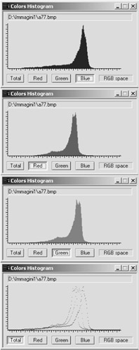
Figure 19.4: Color histograms in RGB space

We first define the concept of an L1-distance on color histograms due to [7].

Definition (L₁ distance) The L₁-norm distance function is

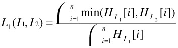
For example, suppose we consider images having 512 colors. In this case, there would be 512 bins for each of the two images I₁, I₂. For each color, we compute the minimum of the number of pixels having that color in image I₁ and I₂. We add all these minima up. The denominator is just the number of pixels in the first image (when both images are of the same size, the denominator is the same irrespective of whether I₁ is considered or I₂ is considered). This function measures nicely the distance between two images. When there is wide variation between the color schemes of the two images, the numerator will be relatively small because for each color, the smaller of the number of pixels in images I₁, I₂ is counted.

Another notion of image distances based on color histograms is the L₂-distance given in [11].

Definition (L₂ distance) The L₂-norm distance function is given by:

A=a[k,t] is an expression that denotes the cross-correlation between histogram bins.

3.1.4.b Texture Distances

It is well known in the literature [12] that color histograms are not sufficient to describe spatial correlations in images. In this section, we describe how textures may be used to define a distance between two images. Texture and shape have been widely analyzed and several features have been proposed [12], [13], [14], [15]. However, all the proposed visual descriptors exploit spatial interactions between a number of pixels in a certain region. In our AVE! system, we have used Wavelet Transform based descriptors in order to provide a multiresolution characterization of the images [16].

Let I be an image defined on a support Ω ⊆ ℜ². Here, Ω is any arbitrary subset of ℜ² . The continuous wavelet transform of I is the functional

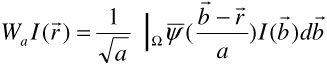
where a is a scaling term and , ∈ Ω. ψ is the 'mother' wavelet satisfying certain regularity constraints. represents the conjugate complex of ψ.

A widely used scheme for image processing applications is Mallat's algorithm [17]. This multiresolution approach is based on the well known subband decomposition technique where an input signal is recursively filtered by perfect reconstruction QMF low-pass and high-pass filters, followed by critical sub-sampling, e.g., subsampling by 2 in the bi-dimensional case [18], [2].

Definition (Wavelet Covariance Signature) A Wavelet Covariance Signature of a given image is the set of real number:

where each is the covariance of an image I:

IDX being the detail subbands of the X component in a given Color Space of an Image I.

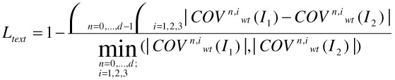
We are now ready to define the texture distance between two images.

Definition (Texture Distance L_text) Given two images I₁ and I₂, the texture distance L_text is defined as

3.1.4.c Shape Distances

Thus far, we have focused on color distances and texture distances. A third type of distance between two images is based on the shapes of the images involved.

It is well known in the computer vision literature that the wavelet transform provides useful information for curvature analysis [19]. The idea is to find corner points and to use them as high curvature points in a polygonal approximation curve of the image. This task may be performed by means of Local Maxima of Wavelet Transform points. In our AVE! system, WT local maxima are calculated by using those points having a WT modulus which is longer than a certain threshold [20].

Definition (Shape Descriptor) A wavelet based shape descriptor is the sequence:

Definition (Shape Distance) Given two images I' and I", and two associated wavelet shape descriptors, and , the wavelet shape distance between I' and I" is given by

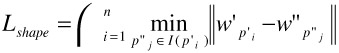
where I(p'_i) = [p'_i -Δp'_i, p'_i+Δp'_i].

3.2 Projection

In the selection operator defined above, visual objects and regions play a role similar to attributes in relational algebra, while blocks play a role similar to tuples in relational algebra. Object properties, accessible via paths, are tested to evaluate selection conditions on blocks in the same way as attribute values are used to select tuples in relational algebra.

The analogy is further enhanced by the Projection operator that we define below. Given a video, whose blocks contain a number of different objects, projection takes as input a specification of the objects that the user is interested in, and deletes from the input video all objects not mentioned in the object specification list. Of course, pixels that in the original video correspond to the eliminated objects must be set to some value. We will introduce the concept of a recoloring strategy that automatically recolors appropriate parts of a video.

To define Projection, we first introduce some notation necessary for the two steps mentioned above.

Object extraction: given a block b, and a list obj-list of objects, object extraction returns a specification of the pixels associated with the objects mentioned in obj-list within block b.

Recoloring: given a block b, a coloring strategy and a specification of a set of pixels, it applies the coloring strategy to all the specified pixels in the block, and returns the newly colored block.

We are now ready to give the definition of projection.

Definition (projection) Suppose v is a video, obj-list is a list of objects from v and Color is a recolor strategy. The projection of obj-list from video v, under recoloring strategy Color, denoted , is given by:

π_{obj-list,Color}(v) = {Color (b, (pixels(b) - Extract (b, obj-list))) | b^∈ v }

We assume that all blocks in π_{obj-list,Color} (v) are ordered in the same way as they were in v, i.e., projection preserves order.

In the above, pixels(b) denotes all pixels in block b, and Extract(b,obj-list) returns all pixels in b that are in an object in obj-list. Thus, pixels(b)-Extract(b,obj-list) refers to all pixels in an image that do not involve any of the objects being projected out. These are the pixels that need to be recolored. This is what the Color function does.

If V is a set of videos, π_{obj-list,Color} (V) = {π_{obj-list,Color}(v)|v ∈ V}

Example. Assume we have a couple of videos, v1 and v2, whose visual objects are cats and dogs. Assume also that we are interested in a new video production, only about dogs. If WHITENING is the coloring strategy that sets to white the specified pixels, π_{<dog>,WHITENING} ({v1, v2}) returns the set containing two videos v1' and v2', each one containing the dogs appearing in the corresponding given video, acting in a completely white environment.

3.3. Cartesian Product

In this section, we define the Cartesian Product of two videos. In classical relational databases, the Cartesian product of two relations R,S simply takes each tuple t in R and t' in S and concatenates them together and places the result in the Cartesian product.

In order to successfully define Cartesian Product of two videos, we need to explain what it means to "concatenate" two blocks together. This is done via the concept of a block merge function.

Definition (block merge function) A block merge function is any function from pairs of blocks to blocks.

There are numerous examples of block merge functions. Three simple examples are given below. We emphasize that these are just three examples of such functions - many more exist.

Example. Suppose f1,f2 are any two frames (from videos v1, v2, respectively). The split-merge, sm(f1, f2), of f1 and f2 is defined as any frame f that shows both f1 and f2. For example,

• [left-right split merge] f's left side may show f1 (in a suitably compressed form) and its right side may show f2.

• [top-down split merge] Alternatively, f's top may show f1, and f's bottom may show f2.

• [embedded split merge] Alternatively, f may most contain frame f1, but a small window at its top left corner may contain a compressed version of f2.

Suppose b = f₁,..,f_m and b' = g₁,…,g_n are two blocks (continuous sequence of frames). Let h_i = sm(f_i,g_i) if i <= min(m,n). If m< n and i > =m, then h_i = g_i. If n < m and i >= n, then h_i = f_i. The split-merge sm(b1,b2) of two blocks is then defined to be the sequence h₁,…,h_max(m,n).

Note that the above are just three examples of how to merge two blocks. Literally hundreds (if not thousands of variants) are possible.

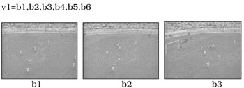
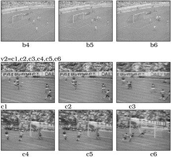
Definition (cartesian product) The Cartesian product, (v₁ X_BM v₂) of two videos v₁=b₁,..,b_m, v₂=c₁,..,c_n, under the block merge function BM consists of the set { BM(bi,cj) | i <= m, j<=n }.

This set is totally ordered under the following ordering. BM(b_i,c_j) <= BM(b_h,c₁) iff either i < h or (i=h AND j <= 1).

Suppose v1= b1,b2 and v2= c1,c2,c3 are two videos. Suppose each block consists of just a single frame. Figure 19.5 shows an example of Cartesian product under left-right, top-down and embedded split merge.

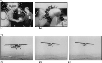
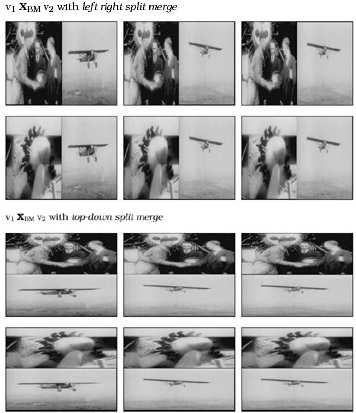
Figure 19.5: Example of Cartesian product

3.4 Join

In classical relational databases, the join of two relations under some join condition C is simply the set of all tuples in the Cartesian product of the two relations that satisfy C. Fortunately, the same is true here.

Definition (join) Suppose v₁,v₂ are two videos, BM is a block merge functio, and C is a selection condition. The join of v₁, v₂ under BM w.r.t. selection condition C, denoted v₁/_Cv₂ consists of the set:

v₁/_Cv₂ = {BM(b₁ ,b₂) | b₁ ∈ v₁ ,b₂ ∈ v₂ ∧ BM(b₁, b₂) |= C}

This set is totally ordered in the same way as defined in the definition of the Cartesian product.

Intuitively, when we join two videos together, we merge the first block in v₁ with all blocks in v₂ when the merge satisfies C, then continue with the second block in v₁ and so on.

Example. v1 join v2 under Embedded Split Merge w.r.t. selection condition: O.ActName: "goal", i.e., v₁/O.ActName="goal" v₂

The selection condition is satisfied by v₅ and c₆; v₆ and c₆.

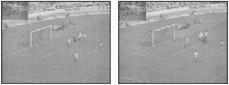
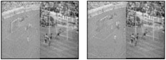
Example. v1 join v2 under Left Right Split Merge w.r.t. selection condition: O.ActName: "goal", i.e., v₁/O.ActName="goal" v₂

3.5 Union, Intersection and Difference

The only complication involved in defining these operations is that we must specify the order of the blocks involved.

Definition (Union, Intersection, Difference) Suppose v₁=b₁,..,b_m, v₂=c₁,..,c_n are two videos.

• The union of v1, v2 is b1,..,bm, c1,..,cn

• The intersection of v₁, v₂ consists of all blocks in v₁ that also occur in v₂. The order of the blocks in v₁ is preserved.

• The difference of v₁, v₂ consists of all blocks in v₁ that are not present in v₂. The order of blocks in v₁ is preserved.

Note that all these operations preserve the order of v₁. Hence, these operations are not symmetric (as is true of standard set theory).