3. User Profiling and Video Exploration

3.1 Definition

Profiling is a business concept from the marketing community, with the aim of building databases that contain the preferences, activities and characteristics of clients and customers. It has long been part of the commercial sector, but which has developed significantly with the growth of e-commerce, the Internet and information retrieval.

The goal of profiling video exploration is to have the most complete picture of the video users we can.

Mining the videos server, which is also achieved using cookies, carries out profiling scenes off-line. The long-term objective is to create associations between potential commercial video sites and commercial marketing companies. These sites make use of specific cookies to monitor a client's explorations at the video site and record data that users may have provided to the exploration server.

User likes, dislikes, browsing patterns and buying choices are stored as a profile in a database without user knowledge or consent.

3.2 Scene Features

We consider a robot named Access that extracts, invisibly, features from video user explorations. Access is synchronized with the playing of a scene that resulted from user browsing or queries.

To enable Access to compile meaningful reports for its client video sites and advertisers and to better target advertising to user, Access collects the following type of non-personally identifiable feature about users who are served via Access technology, User IP address, a unique number assigned to every computer on the Internet. Information, which Access can infer from the IP address, includes the user's geographic location, company and type and size of organization (user domain type, i.e., .com, .net, or .edu.), a standard feature included with every communication sent on the Internet. Information, which Access can infer from this standard feature, includes user browser version and type (i.e., Netscape or Internet Explorer), operating system, browser language, service provider (i.e., Wanado, Club internet or AOL), local time, etc., the manner of using the scene or shot visit within an Access client's site. For example, the features represent instant of start and instant of end of video scene the user views. Affiliated advertisers or video publishers may provide access with non-personally identifiable demographic features so that user may receive ads that more closely match his interests. This feature focuses on privacy protections as the access-collected non-personally identifiable data. Access believes that its use of the non-personally identifiable data benefits the user because it eliminates needless repetition and enhances the functionality and effectiveness of the advertisements the users view which are delivered through the Access technology.

The feature collected is non-personally identifiable. However, where a user provides personal data to a video server, e.g., name and address, it is, in principle, possible to correlate the data with IP addresses, to create a far more personalized profile.

3.3 Mathematical Modeling

Given the main problem "profiling of video exploration," the next step is the selection of an appropriate mathematical model. Numerous time-series prediction problems, such as in [24], supported successfully probabilistic models. In particular, Markov models and Hidden Markov Models have been enormously successful in sequence generation. In this paper, we present the utility of applying such techniques to prediction of video scene explorations.

A Markov model has many interesting properties. Any real world implementation may statistically estimate it easily. Since the Markov model is also generative, its implementation may derive automatically the exploration predictions. The Markov model can also be adapted on the fly with an additional user exploration feature. When used in conjunction with a video server, this later may use the model to predict the probability of seeing a scene in the future given a history of accessed scenes. The Markov state-transition matrix represents, basically, "user profile" of the video scene space. In addition, the generation of predicted sequences of states necessitates vector decomposition techniques.

Markov model creations depend on an initial table of sessions in which each tuple corresponds to a user access.

 INSERT INTO [Session] ( id, idsceneInput ) SELECT[InitialTable].[Session_ID], [InitialTable].[Session_First_Content] FROM OriginalTable GROUP BY [InitialTable].[Session_ID], [InitialTable].[Session_First_Content] ORDER BY [InitialTable].[Session_ID];

3.4 Markov Models

A set of three elements defines a discrete Markov model:

α corresponds to the state space. β is a matrix representing transition probabilities from one state to another. λ is the initial probability distribution of the states in α.

Each transition contains the identification of the session, the source scene, the target scene and the dates of accesses. This is an example of transition table creation.

 SELECT     regroupe.Session_ID,      regroupe.Content_ID     AS     idPageSource, regroupe.datenormale   AS   date_source,   regroupe2.Content_ID   AS  idPageDest, regroupe2.datenormale AS date_dest INTO transitions FROM [2)  regroupe sessions from call4]  AS regroupe,  [2) regroupe sessions from call4] AS regroupe2 WHERE               (((regroupe2.Session_ID)=regroupe!Session_ID)             And ((regroupe2.Request_Sequence)=regroupe!Request_Sequence+l));

The fundamental property of Markov model is the dependencies of the previous states. If the vector α [ι] denotes the probability vector for all the states at time 'ι', then:

If there are 'ℵ' states in the Markov model, then the matrix of transition probabilities β is of size ℵ x ℵ. Scene sequence modeling supports Markov model. In this formulation, a Markov state corresponds to a scene presentation, after a query or a browsing.

Many methods estimate the matrix β. Without loss of generality, the maximum likelihood principle is applied in this paper to estimate β and λ. The estimation of each element of the matrix λ [v, v'] respect the following formula:

ϕ (v, v') is the count of the number of times v' follows v in the training data. We utilize the transition matrix to estimate short-term exploration predictions. An element of the matrix state, say λ [v, v'], can be interpreted as the probability of transitioning from state v to v' in one step. Similarly, an element of α*α will denote the probability of transitioning from one state to another in two steps, and so on.

Given the "exploration history" of the user ξ (ι-κ), ξ (ι-κ+1).… ξ (ι-1), we can represent each exploration step as a vector with a probability 1 at that state for that time (denoted by τ (ι-κ), τ (ι-κ+1)… τ (ι-1)). The Markov model represents estimation of the probability of being in a state at time 'ι' is shown in:

The Markovian assumption varies in different ways. In our problem of exploration prediction, we have the user's history available. Answering to which of the previous explorations are "good predictors" for the next exploration creates the probability distribution. Therefore, we propose variants of the Markov process to accommodate weighting of more than one history state. So, each of the previous explorations are used to predict the future explorations, combined in different ways. It is worth noting that rather than compute λ*λ and higher powers of the transition matrix, these may be directly estimated using the training data. In practice, the state probability vector α (ι) can be normalized and compared against a threshold in order to select a list of "probable states" that the user will choose.

3.5 Predictive Analysis

The implementation of Markov models into a video server makes possible four operations directly linked to predictive analysis.

In the first one, the server supports Markov models in a predictive mode. Therefore, when the user sends an exploration request to the video server, this later predicts the probabilities of the next exploration requests of the user. This prediction depends on the history of user requests. The server can also support Markov models in an adaptive mode. Therefore, it updates the transition matrix using the sequence of requests that arrive at the video server.

In the second one, prediction relationship, aided by Markov models and statistics of previous visits, suggests to the user a list of possible scenes, of the same or different video bases, that would be of interest to him, and then the user can go to the next. The prediction probability influences the order of scenes. In the current framework, the predicted relationship does not strictly have to be a scene present in the current video base. This is because the predicted relationships represent user traversal scenes that could include explicit user jumps between disjoint video bases.

In the third one, there is generation of a sequence of states (scenes) using Markov models that predict the sequence of states to visit next. The result returned and displayed to the user consists of a sequence of states. The sequence of states starts at the current scene the user is browsing. We consider default cases, such as, if the sequence of states contains cyclic state, they are marked as "explored" or "unexplored." If multiple states have the same transition probability, a suitable technique chooses the next state. This technique considers the scene with the shortest duration. Finally, when the transition probabilities of all states from the current state are too weak, then the server suggests to the user the come back to the first state.

In the fourth one, we refer to video bases that are often good starting points to find documents, and we refer to video bases that contain many useful documents on a particular topic. The notion of profiled information focuses on specific categories of users, video bases and scenes. The video server iteratively estimates the weights of profiled information based on the Markovian transition matrix.

3.6 Path Analysis and Clustering

To reduce the dimensionality of the Markov transition matrix β, a clustering approach is used. It reduces considerably the number of states by clustering similar states into "similar groups." The originality of the approach is to discover automatically the number of clusters. The reduction obtained is about log ℵ, where ℵ is the number of scenes before clustering.

3.6.1 How to discover the number of clusters: k

A critical question in the partition clustering method is the number of clusters (k). In the majority of real world experimented methods, the number of cluster k is manually estimated. The estimation needs a minimum knowledge on both data databases and applications, and this requires the study of data. Bad values of k can lead to very bad clustering. Therefore, automatic computation of k is one of the most difficult problems in cluster analysis.

To deal with this problem, we consider a method based on the confidence measures of the clustering. To compute the confidence of the clustering, we consider together two-levels of measures: the global level and the local level. Global Variance Ratio Criterion measure (GVRC) inspired of [4] underlines the global level, and Local Variance Ratio Criterion (LVRC) inspired of [9] measure underlines the local level. GVRC has been never used in partition clustering. It computes the confidence of the whole clusters, and LVRC computes the confidence of individual clusters, known also by silhouette. Therefore, we combine the two levels of measures to correct the computation of the clustering confidence.

Our choices of GVRC and LVRC confidence measures are based on the following arguments. Previous experiments, in [13], in the context of hierarchical clustering, examined thirty measures in order to find the best number of clusters. They apply all of them to a test data set, and compute how many times an index gives the right k. GVRC measure presented the best results in all cases, and GVRCN normalizes GVRC measure (GVRCN value is between 0 and 1). The legitimate questions may be: how is this measure (GVRC) good for partition methods? GVRC is a good measure for hierarchical methods. Is GVRC also good for partition methods? Are there any direct dependencies between data sets (in our case image descriptors) and the confidence of clustering measures? What are relationships between the initial medoids and the measures of the confidence of clustering?

It is too hard to answer all these questions in the same time without theory improvements and exhaustive real world experiments. Therefore, our approach objective is not to answer accurately to all these important questions, but to contribute to these answers by presenting results of a real world experiment. We extend a measure of clustering confidence, by considering the best one presented in the literature [13]. Then, we experimented this measure in our state space.

As said a few lines ago, we combine the two levels of measures to accurate the computation of the clustering confidence. The combination of two levels of measures is an interesting particularity of our method. It avoids the clustering state where the max value of average confidence of clusters does not mean the best confidence of clustering. The method is improved by identifying the best cluster qualities with the lowest variance.

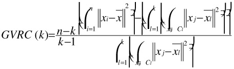
GVRC is described by the following formula.

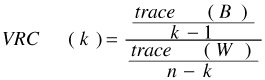
n is the cardinality of the data set. K is the number of clusters. Trace(B)/(k-1) is the dispersion (variance) between clusters. Trace (W)/n-k is the dispersion within clusters. The expanded formula is:

click to expand

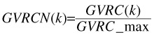
The best clustering coincides with the maximum of GVRC. To normalize the GVRC value (0≤GVRCN≤1), we compute GVRCNormalized (GVRCN), where GVRC_max = GVRC (k'), and ∀ k, 0 < k ≤ k_max, k ≠ k', GVRC (k) < GVRC (k'). K_max is the maximum of cluster considered. K_max ≤ the cardinal of the data items.

Local Ratio Criterion (LVRC) measures the confidence of the clusterj (C_j). The formula is:

click to expand

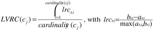
lvrc measures the probability of x_i to belong to the cluster C_xi, where a_xi is the average dissimilarity of object x_i to all other objects of the cluster C_xi and b_xi is the average dissimilarity of object x_i to all objects of the closest cluster C'_xi (neighbor of object x_i). Note that the neighbor cluster is like the second-best choice for object x_i. When cluster C_xi contains only one object x_i, the s_xi is set to zero (lvrc_xi= 0).

3.6.2 K-automatic discovery algorithm

The algorithm is run several times with different starting states according to different k values, and the best configuration of k obtained from all runs is used as the output clustering.

We consider the sequence variable sorted_clustering initialized to empty sequence (< >). sorted_clustering contains a sorted, on basis of confidencei, sequence of elements in the form of <confidence_i,k_i> where k_i is the cluster number at i iteration and confidence_i is the global variance ratio criterion and all local variance ratio criterion associated to k_i clusters. sorted_clustering = <….., <confidence_i-1,k_i-1>, <confidence_i,k_i>>, where confidence_i = <GVRC(k), <LVRC(c₁), LVRC(c₂), …., LVRC(c_ki)> >.

The algorithm follows five steps:

The first one initializes the maximum number of k authorized (max_k), by default max_k = n/2. n is the number of data items.

The second step applies the clustering algorithm at each iteration k_i (for k=1 to max_k), computes GVRC(k) and, for each k value, computes LVRC(c_j), for j = 1, .., k. confidence_i = < GVRC(k),<LVRC(c₁), LVRC(c₂), …., LVRC(c_k)> >.

 K-discovery() { Set max_k //By default max_k = n/2 sorted_clustering ← < > /* empty sequence */ sorted_clustering  contains  a sequence  of  sorted  qualities  of  clustering  and associated k. sorted_clustering = <….., <confidence_i-1,k_i-1>, <confidence_i,k_i>>, where confidence_i-1 < confidence_i-1 <confidence_i,k_i> = <GVRC(k_i), k_i> // The clustering confidence is often the best when the value is high. for k=1 to max_k do   Apply chosen clustering algorithm. Current ← GVRC (k) , <LVRC (c₁) , LVRC (c₂), …., LVRC(c_k) > /* GVRC(k) = confidence of actual clustering */ sorted_clustering ← insert <k, current> in best_clustering, by considering sorted sequence of sorted_clustering.  end for GVRC_max ←•max_confidence (sorted_clustering) /* GVRC_max = best_clustering */ correct_sorted_clustering ←•< > for k=1 to max_k do   if 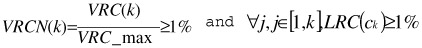   then /* C_k is a correct cluster */      correct_sorted_clustering      ←      insert      <k,       confidence_k>     in correct_sorted_clustering>   end if end for if correct_sorted_clustering = <> then { for i=1 to cardinal(correct_sorted_clustering) do { moving false or weak data items of C_ij for which LRC(c_ikj)<1% to Noisy_cluster if cardinal (Noisy_cluster) < 10% then k-discovery() without considering the noisy data items in Noisy Class } Return correct_sorted_clustering. }

The third step normalizes the global variance ratio criterion (GVRC), by computing global variance ratio criterion normalized (GVRCN). GVRC_max = max_GVRC(k) where GVRC_max corresponds to the best_clustering.

The fourth step considers only k clustering for which GVRCN(k) = GVRC(k)/GVRC_max is the minimum value and LVRC(k) is the maximum. So, 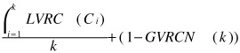is the maximum, and ∀j,j∈[l,k],LVRC(c_k)≥l%. The results are sorted in correct_sorted_clustering. If the final correct_sorted_clustering is not empty, therefore, we have at least one solution and the algorithm is stopped. If not, the current step is followed by the fifth step.

The fifth step looks for false or weak clusters (LVRC < 1 %). All false or weak data items of these false or weak clusters are moved in a specific cluster, called "Noisy cluster." If the cardinality of the Noisy cluster is less than 10% then we compute the k-discovery without considering the false or weak data items.

However, if the cardinal of the Noisy cluster is greater than 10%, then we consider that there are too many noises and the data item features of the initial databases should be reconsidered before applying again the k-discovery algorithm. We deduce that the data item descriptors are not suited to clustering analysis.

3.6.3 Clustering algorithm

The clustering algorithm is a variant of k-medoids, inspired of [16]. The particularity of the algorithm is the replacement of sampling by heuristics. Sampling consists of finding better clustering by changing one medoid. However, finding the best pair (medoid, item) to swap is very costly (O (k (n-k) ²)).

 Clustering() { Initialize num_tries and num_pairs min_cost ← big_number for k=1 to num_tries do   current ← k randomly selected items in the entire data set.   1 ← 1   repeat     xi ← a randomly selected item in current     xh ← a randomly selected item in {entire data set current} .     if TCih <0 then       current ← currentxi+xh     else       j ← j+1     end if   until j• num_pairs   if min_cost < cost(current) then     best ← current .   end if end for Return best. }

That is why heuristics have been introduced in [16] to improve the confidence of swap (medoid, data item). To speed up the choice of a pair (medoid, data item), the algorithm sets a maximum number of pairs to test (num_pairs), then chooses randomly a pair and compares the dissimilarity (the comparison is done by evaluating TC_ih).

If this dissimilarity is greater than the actual dissimilarity, just go on choosing pairs until the number of pairs chosen reaches the maximum fixed. The medoids found are very dependent of the k first medoids selected. So the approach selects k other items and restarts num_tries times (num_tries is fixed by user). The best clustering is kept after the num_tries tries.