Making Workbooks Easier to Work With | MicrosoftВ® Office ExcelВ® 2003 Step by Step (Step By Step (Microsoft))

An important component of making workbooks easy to work with is to give users an idea of where to find the data they re looking for. Excel provides several ways to set up signposts directing users toward the data they want. The first method is to give each workbook a descriptive name. Once users have opened the proper workbook, you can guide them to a specific worksheet by giving each worksheet a name ; the names are displayed on the sheet tabs in the lower-left corner of the workbook window. To change a worksheet s name, you right-click the sheet tab of the worksheet you want and, from the shortcut menu that appears, choose Rename. Choosing Rename opens the worksheet name for editing. You can also change the order of worksheets in a workbook by dragging the sheet tab of a worksheet to the desired position on the navigation bar, bringing the most popular worksheets to the front of the list.

If you need more than three worksheets in most of the workbooks you create, you can change the default number of worksheets in your new workbooks. To change the default number of worksheets, on the Tools menu, click Options. In the Options dialog box, click the General tab, and, in the Sheets In New Workbook box, type the number of worksheets you want in your new workbooks, and click OK.

After you have put up the signposts that make your data easy to find, you can take other steps to make the data in your workbooks easier to work with. For instance, you can change the width of a column or the height of a row in a worksheet by dragging the column or row s border to the desired position. Increasing a column s width or a row s height increases the space between cell contents, making it easier to select a cell s data without inadvertently selecting data from other cells as well.

Tip

You can apply the same change to more than one row or column by selecting the rows or columns you want to change and then dragging the border of one of the selected rows or columns to the desired location. When you release the mouse button, all of the selected rows or columns will change to the new height or width.

Modifying column width and row height can make a workbook s contents easier to work with, but you can also insert a row or column between the edge of a worksheet and the cells that contain the data to accomplish this as well. Adding space between the edge of a worksheet and cells, or perhaps between a label and the data to which it refers, makes the workbook s contents less crowded and easier to work with. You insert rows by clicking a cell and then, on the Insert menu, clicking Rows. Excel inserts a row above the active cell. You insert a column in much the same way by clicking Columns on the Insert menu. When you do this, Excel inserts a column to the left of the active cell.

Likewise, you can insert individual cells into a worksheet. To insert a cell, click the cell that is currently in the position where you want the new cell to appear, and on the Insert menu, click Cells to display the Insert dialog box. In the Insert dialog box, you can choose whether to shift the cells surrounding the inserted cell down (if your data is arranged as a column) or to the right (if your data is arranged as a row). When you click OK, the new cell appears, and the contents of affected cells shift down or to the right, as appropriate. In a similar vein, if you want to delete a block of cells, select the cells, and on the Edit menu, click Delete to display the Delete dialog box, complete with option buttons that let you choose how to shift the position of the cells around the deleted cells.

Tip	The Insert dialog box also includes option buttons you can select to insert a new row or column; the Delete dialog box has similar buttons that let you delete an entire row or column.

In some cases, the values you want to put in the new cells might already exist in your worksheet. For example, Catherine Turner might have typed some sales data into a blank worksheet in anticipation of modifying the sheet once the rest of the data was entered. You can move cells from another part of your worksheet, rather than just copy or cut the values from the cells and paste them into other cells, by using a variation of the standard cut-and-paste operation. After you select the cells and click the Cut toolbar button on the Standard toolbar, on the Insert menu, click Cut Cells. The Insert Paste dialog box will appear, allowing you to choose how to shift the cells surrounding the cells you re inserting.

Tip	If you click the Copy toolbar button instead of the Cut toolbar button, the menu item on the Insert menu will be Copy Cells instead of Cut Cells.

Sometimes adding cells or even changing a row s height or a column s width isn t the best way to improve your workbook s usability. For instance, even though a column label might not fit within a single cell, increasing that cell s width (or every cell s width) might throw off the worksheet s design. While you can type individual words in cells so that the label fits in the worksheet, another alternative is to merge two or more cells. Merging cells tells Excel to treat a group of cells as a single cell as far as content and formatting go. To merge cells into a single cell, you click the Merge and Center toolbar button. As the name of the button implies, Excel centers the contents of the merged cell.

Tip	Clicking a merged cell and then clicking the Merge and Center toolbar button removes the merge.

If you want to delete a row or column, you right-click the row or column head and then, from the shortcut menu that appears, click Delete. You can temporarily hide a number of rows or columns by selecting those rows or columns and then, on the Format menu, pointing to Row or Column and then clicking Hide. The rows or columns you selected disappear, but they aren t gone for good, as they would be if you d used Delete. Instead, they have just been removed from the display until you call them back; to return the hidden rows to the display, on the Format menu, pointto Row or Column and then click Unhide.

When you insert a row, column, or cell in a worksheet with existing formatting, the Insert Options button appears. As with the Paste Options button and the Auto Fill Options button, clicking the Insert Options button displays a list of choices you can make about how the inserted row or column should be formatted. The options are summarized in the following table:

Option	Action
Format Same as Above	Apply to the inserted row the formatting of the row above it.
Format Same as Below	Apply to the inserted row the formatting of the row below it.
Format Same as Left	Apply to the inserted column the formatting of the column to its left.
Format Same as Right	Apply to the inserted column the formatting of the column to its right.
Clear Formatting	Apply the default format to the new row or column.

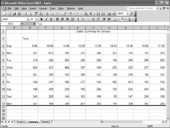
In this exercise, you make the worksheet containing last January s sales data easier to read. First you name the worksheet and bring it to the front of the list of worksheets in its workbook. Next you increase the column width and row height of the cells holding the sales data. In addition, you merge and center the worksheet s title and then add a row between the title and the row that holds the times for which The Garden Company recorded sales. Then you add a column to the left of the first column of data and then hide rows containing data for all but the first week of the month.

BE SURE TO start Excel before beginning this exercise.

USE the Easier.xls document in the practice file folder for this topic. This practice file is located in the My Documents\Microsoft Press\Office 2003 SBS\SettingUpWorkbook folder, and can also be accessed by clicking Start/All Programs/Microsoft Press/Microsoft Office System 2003 Step by Step .

OPEN the Easier.xls document.

Select cells C1 to D3 and, on the Standard toolbar, click the Cut button.
Select cells B5 to C7.
On the Insert menu, click Cut Cells .

The Insert Paste dialog box appears.
If necessary, select the Shift Cells Right option, and click OK .

The cut cells appear in cells B5 to C7, pushing the existing cells to the right. The values in cells C5 to C7 are repeated incorrectly in cells D5 to D7.
Select cells D5 to D7 and, on the Edit menu, click Delete .

The Delete dialog box appears.
If necessary, select the Shift Cells Left option, and click OK .

Cells D5 to D7 are deleted.
In the lower-left corner of the workbook window, right-click the Sheet2 sheet tab.
From the shortcut menu that appears, click Rename .

Sheet2 is highlighted.
Type January , and press [ENTER].

The name of the worksheet changes from Sheet2 to January .
Click the January sheet tab, and drag it to the left of the Sheet1 sheet tab.

The January sheet tab moves to the left of the Sheet1 sheet tab. As the sheet tab moves, an inverted black triangle marks the sheet s location in the workbook.
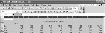
Click the column head for column A, and drag to column M.

Columns A through M are highlighted.
Position the mouse pointer over the right edge of column A, and drag the edgeto the right until the ScreenTip reads Width: 10.00 (75 pixels) .

The width of the selected columns changes.
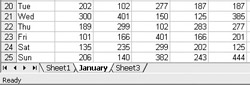
Select rows 3 through 35.

Rows 3 through 35 are highlighted.
Position the mouse pointer over the bottom edge of row 3, and drag the edge down until the ScreenTip says Height: 25.50 (34 pixels) .

The height of the selected rows changes.
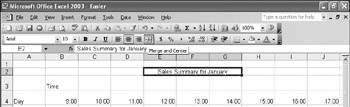
Click cell E2, and drag to cell G2.

On the Formatting toolbar, click the Merge and Center toolbar button.

Important

Depending on the screen resolution you have set on your computer and which toolbar buttons you use most often, it s possible that not every button on every toolbar will appear on your Excel toolbars . If a button mentioned in this book doesn t appear on a toolbar, click the Toolbar Options down arrow on that toolbar to display the rest of the buttons available on that toolbar.

Cells E2, F2, and G2 are merged into a single cell, and the new cell s contents are centered.

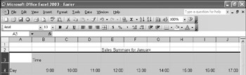
Click cell A3.
On the Insert menu, click Rows .

A new row, labeled row 3, appears above the row previously labeled row 3.
On the Insert menu, click Columns .

A new column, labeled column A, appears to the left of the column previously labeled column A.
Select rows 13 through 36.

Rows 13 through 36 are highlighted.
On the Format menu, point to Row , and then click Hide .

Rows 13 through 36 disappear from the worksheet.
On the Format menu, point to Row , and then click Unhide .

The hidden rows reappear in the worksheet.
On the Tools menu, click Options .

The Options dialog box appears.
Click the General tab.

The General tab page appears.
In the Sheets In New Workbook box, type 12 .
Click OK .
On the Standard toolbar, click the Save button.

Excel saves the document.

CLOSE the Easier.xls document.