Formatting PivotTables

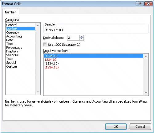
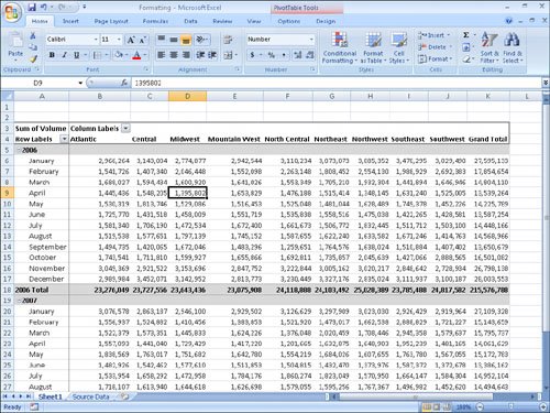
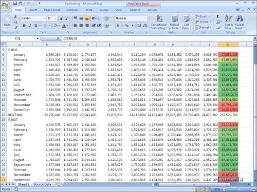
PivotTables are the ideal tools for summarizing and examining large data tables, even those containing in excess of 10 or even 100,000 rows. Even though PivotTables often end up as compact summaries, you should do everything you can to make your data more comprehensible. One way to improve your data's readability is to apply a number format to the PivotTable Values field. To apply a number format to a field, right-click any cell in the field and then click Number Format to display the Format Cells dialog box. Select or define the format you want to apply and then click OK to enact the change.

See Also

For more information on selecting and defining cell formats by using the Format Cells dialog box, see "Formatting Cells" in Chapter 5.

Analysts often use PivotTables to summarize and examine organizational data with an eye to making important decisions about the company. For example, chief operating officer Jenny Lysaker might examine monthly package volumes handled by Consolidated Messenger and notice that there's a surge in package volume during the winter months in the United States.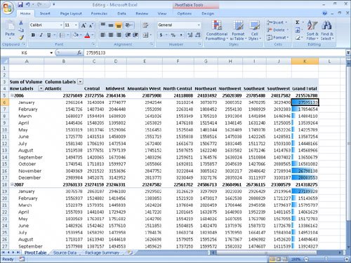

Excel 2007 extends the capabilities of your PivotTables by enabling you to apply a conditional format to the PivotTable cells. What's more, you can select whether to apply the conditional format to every cell in the Values area, to every cell at the same level as the selected cell (that is, a regular data cell, a subtotal cell, or a grand total cell) or to every cell that contains or draws its values from the selected cell's field (such as the Volume field in the previous example).

To apply a conditional format to a PivotTable field, click a cell in the Values area. On the Home tab, in the Styles group, click Conditional Formatting and then create the desired conditional format. After you do, Excel 2007 displays a Formatting Options smart tag, which offers three options on how to apply the conditional format:

• Selected cells, which applies the conditional format to the selected cells only

• All cells showing "Sum of field_name" values, which applies the conditional format to every cell in the data area, regardless of whether the cell is in the data area, a subtotal row or column, or a grand total row or column

• All cells showing "Sum of field_name" values for fields, which applies the conditional format to every cell at the same level (for example, data cell, subtotal, or grand total) as the selected cells

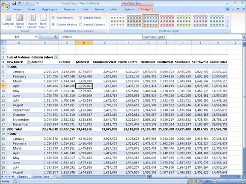
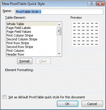
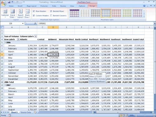
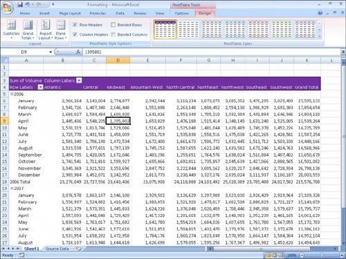
See Also

For more information on creating conditional formats, see "Changing the Appearance of Data Based on Its Value" in Chapter 5.

In Excel 2003 and earlier versions of the program, you were limited to a small number of formatting styles, called autoformats, which you could apply to a PivotTable. In Excel 2007, you can take full advantage of the Microsoft Office system enhanced formatting capabilities to apply existing formats to your PivotTables. Just as you can create data table formats, you can also create your own PivotTable formats to match your organization's desired color scheme.

To apply a PivotTable style, click any cell in the PivotTable and then, on the Design contextual tab, in the PivotTable Styles group, click the gallery item representing the style you want to apply. If you want to create your own PivotTable style, click the More button in the PivotTable Styles gallery (in the lower-right corner of the gallery) and then click New PivotTable Style to display the New PivotTable QuickStyle dialog box.

Type a name for the style in the Name field, click the first table element you want to customize, and then click Format. Use the controls in the Format Cells dialog box to change the element's appearance. After you click OK to close the Format Cells dialog box, the New PivotTable Quick Style dialog box Preview pane displays the style's appearance. If you want Excel 2007 to use the style by default, select the Set as default PivotTable quick style for this document check box. After you finish creating your formats, click OK to close the New PivotTable Quick Style dialog box and save your style.

The Design contextual tab contains many other tools you can use to format your PivotTable, but one of the most useful is the Banded Columns check box, which you can find on the Design contextual tab, in the PivotTable Style Options group. If you select a PivotTable Style that offers banded rows as an option, selecting the Banded Rows check box turns banding on. If you prefer not to have Excel 2007 band the rows in your PivotTable, clearing the check box turns banding off.

In this exercise, you'll apply a number format to a PivotTable values field, apply a PivotTable style, create your own PivotTable style, give your PivotTable banded rows, and apply a conditional format to a PivotTable.

USE the Formatting workbook in the practice file folder for this topic. This practice file is located in the My Documents\Microsoft Press\Excel SBS\PivotTables folder.

OPEN the Formatting workbook.

1.	On the PivotTable worksheet, right-click any data cell and then click Number Format. The Format Cells dialog box appears.
2.	In the Category list, click Number. The Number tab page appears.
3.	In the Decimal places field, type 0.
4.	Select the Use 1000 Separator (,) check box.
5.	Click OK. Excel 2007 reformats your PivotTable data.
6.	If necessary, on the Design contextual tab, in the PivotTable Style Options group, select the Banded Rows check box.
7.	On the Design contextual tab, in the PivotTable Styles group, click the third style from the left (when you point your mouse pointer to it, Excel 2007 displays a ScreenTip that reads Pivot Style Light 2). Excel 2007 applies the PivotTable style.
8.	On the Design contextual tab, in the PivotTable Styles group, click the More button in the lower-right corner of the style gallery. The gallery expands.
9.	Click New PivotTable Style. The New PivotTable Quick Style dialog box appears.
10.	In the Name field, type Custom Style 1.
11.	In the Table Element list, click Header Row and then click Format. The Format Cells dialog box appears.
12.	On the Font tab, click the Color field down arrow and then click the white square.
13.	On the Border tab, in the Presets area, click Outline.
14.	On the Fill tab, in the Background Color area, click the purple square at the lower-right corner of the color palette.
15.	Click OK. The Format Cells dialog box disappears, and the style change appears in the Preview pane of the New PivotTable Quick Style dialog box.
16.	In the Table Element list, click Second Row Stripe and then click Format. The Format Cells dialog box appears.
17.	On the Fill tab, in the middle part of the Background Color section, click the eighth square in the second row (it's a light, dusty purple).
18.	Click OK twice. The Format Cells dialog box disappears, and your format appears in the PivotTable Styles gallery.
19.	Click the new style. Excel 2007 formats your PivotTable using your custom PivotTable style.
20.	On the Design contextual tab, in the PivotTable Style Options group, clear the Banded Rows check box. Excel 2007 removes the banding from your PivotTable.
21.	Select the cell ranges K6:K17 and K20:K31.
22.	On the Home tab, in the Styles group, click Conditional Formatting, point to Color Scales, and then click the second color scale in the top row (it's a three-color scale with red at the top). Excel 2007 applies the conditional format to the selected cells.

CLOSE the Formatting workbook.