Analyzing Data Dynamically with PivotTables

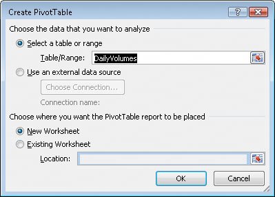
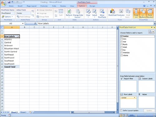
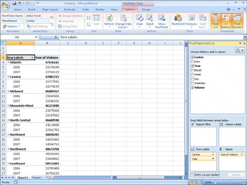
Excel 2007 worksheets enable you to gather and present important data, but the standard worksheet can't be changed from its original configuration easily. As an example, consider the worksheet in the following graphic.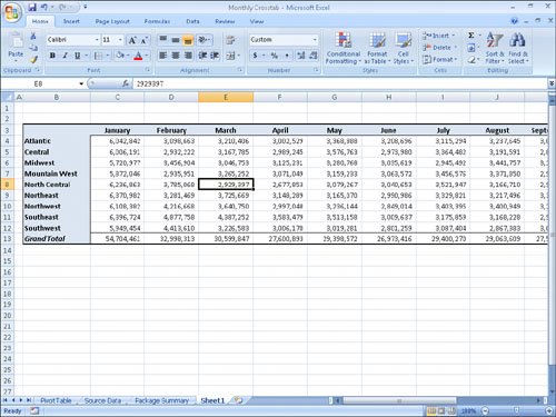

This worksheet records monthly package volumes for each of nine distribution centers in the United States. The data in the worksheet is organized so that each row represents a distribution center, whereas the columns in the body of the worksheet represent a month of the year. When presented in this arrangement, the monthly totals for all centers and the yearly total for each distribution center are given equal billing: neither set of totals stands out.

Such a neutral presentation of your data is versatile, but it has limitations. First, although you can use sorting and filtering to restrict the rows or columns shown, it's difficult to change the worksheet's organization. For example, in a standard worksheet you can't reorganize the contents of your worksheet so that the hours are assigned to the rows and the distribution centers are assigned to the columns.

The Excel 2007 tool to reorganize and redisplay your data dynamically is the PivotTable. You can create a PivotTable, or dynamic worksheet, that enables you to reorganize and filter your data on the fly. For instance, you can create a PivotTable with the same layout as the worksheet shown previously, which emphasizes totals by month, and then change the PivotTable layout to have the rows represent the months of the year and the columns represent a distribution center. The new layout emphasizes the totals by regional distribution center, as shown in the following graphic.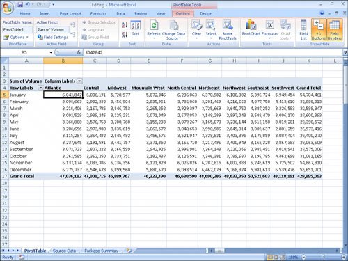

To create a PivotTable, you must have your data collected in a list. The new Excel 2007 data tables mesh perfectly with PivotTable® dynamic views; not only do the data tables have a well-defined column and row structure but the ability to refer to a data table by its name also greatly simplifies PivotTable creation and management.

The following graphic shows the first few lines of the data table used to create the PivotTable just shown.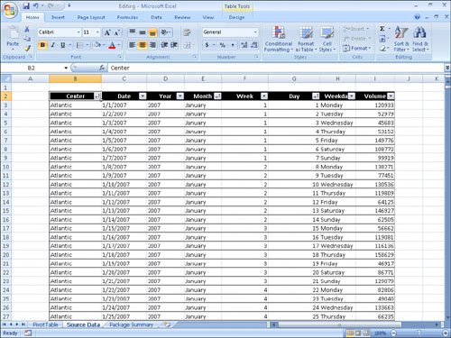

Notice that each line of the table contains a value representing the Distribution Center, Date, Month, Week, Weekday, Day, and Volume for every day of the years 2006 and 2007. Excel 2007 needs that data when it creates the PivotTable so that it can maintain relationships among the data. If you want to filter your PivotTable so that it shows all package volumes on Thursdays in January, for example, Excel 2007 must be able to identify January 11 as a Thursday.

After you create a data table, you can click any cell in that list, display the Insert tab of the user interface, and then, in the Tables group, click PivotTable to display the Create PivotTable dialog box.

In this dialog box, you verify the data source for your PivotTable and whether you want to create a PivotTable on a new worksheet. After you click OK, Excel 2007 creates a new worksheet and displays the PivotTable Field List task pane.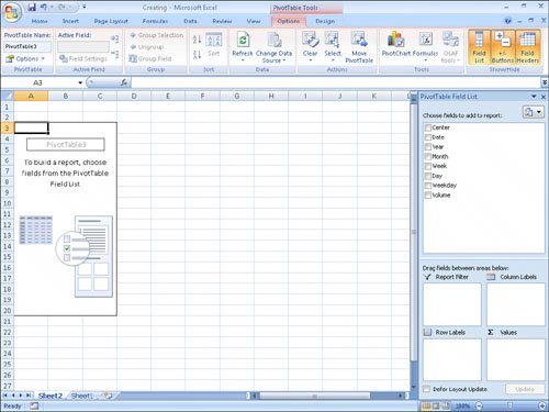

Tip

You should always place your PivotTable on its own worksheet to avoid unwanted edits and reduce the number of cells Excel 2007 must track when you rearrange your data. You might not notice a difference with a small data set, but it's noticeable when your table runs more than a few hundred rows.

To assign a field, or column in a data list, to an area of the PivotTable, drag the field head from the Choose Fields To Add To Report area at the top of the PivotTable Field List task pane to the Drag Fields Between Areas Below area at the bottom of the task pane. For example, if you drag the Volume field header to the Values area, the PivotTable displays the total of all entries in the Volume column.

If the PivotTable Field List task pane isn't visible, click any cell in the PivotTable to display it. If you accidentally click the Close button at the upper-right corner of the PivotTable Field List task pane, you can redisplay the task pane by clicking any cell in the PivotTable to display the PivotTable Tools context tabs on the user interface. On the Options contextual tab, in the Show/Hide group, click Field List.

It's important to note that the order in which you enter the fields in the Row Labels and Column Labels areas affects how Excel 2007 organizes the data in your PivotTable. As an example, the following graphic shows a PivotTable that groups the PivotTable rows by distribution center and then by month.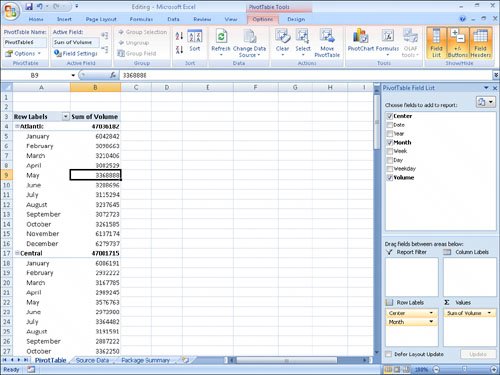

And here is the same PivotTable data, but this time it's organized by month and then by distribution center.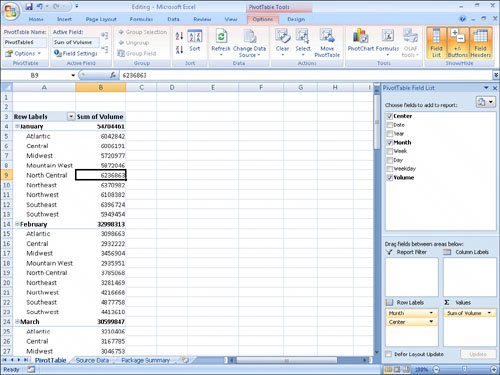

In the preceding examples, all the field headers are in the Row Labels area. If you drag the Center header from the Row Labels area to the Column Labels area, the PivotTable reorganizes its data (pivots) to form this configuration.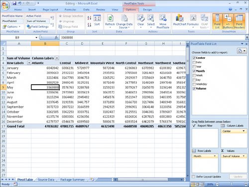

To pivot a PivotTable, you drag a field header to a new position in the PivotTable Field List task pane. As you drag the task pane, Excel 2007 displays a blue line in the interior of the target area so you know where the field will appear when you release the left mouse button. If your data set is large or if you based your PivotTable on a data collection on another computer, it might take some time for Excel 2007 to reorganize the PivotTable after a pivot. You can have Excel 2007 delay redrawing the PivotTable by selecting the Defer Layout Update button at the lower-left corner of the PivotTable Field List task pane. When you're ready for Excel 2007 to display the reorganized PivotTable, click Update.

If you expect your PivotTable source data to change, such as when you link to an external database that records shipments or labor hours, ensure that your PivotTable summarizes all the available data. To do that, you can refresh the PivotTable connection to its data source. If Excel 2007 detects new data in the source table, it updates the PivotTable contents accordingly. To refresh your PivotTable, click any cell in the PivotTable and then, in the Data group, on the Options contextual tab, click Refresh.

In this exercise, you create a PivotTable using data from a table, add fields to the PivotTable, and then pivot the PivotTable.

USE the Creating workbook in the practice file folder for this topic. This practice file is located in the My Documents\Microsoft Press\Excel SBS\PivotTables folder.

BE SURE TO start Excel 2007 before beginning this exercise.

OPEN the Creating workbook.

1.	Click any cell in the data table.
2.	On the Insert tab, in the Tables group, click PivotTable. The Create PivotTable dialog box appears.
3.	Verify that the DailyVolumes table name appears in the Table/Range field and that the New Worksheet option button is selected.
4.	Click OK. Excel 2007 creates a PivotTable on a new worksheet.
5.	In the PivotTable Field List task pane, drag the Center field header to the Row Labels area. Excel 2007 adds the Center field values to the PivotTable row area.
6.	In the PivotTable Field List task pane, drag the Year field header to the Column Labels area. Excel 2007 adds the Year field values to the PivotTable column area.
7.	In the PivotTable Field List task pane, drag the Volume field header to the Values area. Excel 2007 fills in the body of the PivotTable with the Volume field values.
8.	In the PivotTable Field List task pane, in the Column Labels area, drag the Year field header to the Row Labels area and drop it beneath the Center field header. Excel 2007 changes the PivotTable to reflect the new organization.

CLOSE the Creating workbook.