Changing the Appearance of Data Based on Its Value

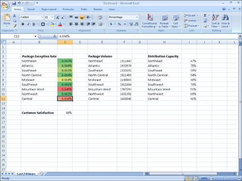
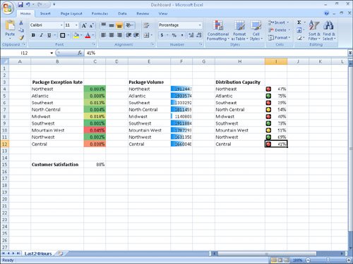
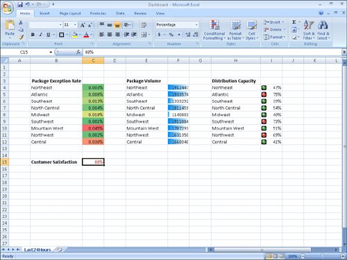
Recording package volumes, vehicle miles, and other business data in a worksheet enables you to make important decisions about your operations. And as you saw earlier in this chapter, you can change the appearance of data labels and the worksheet itself to make interpreting your data easier.

Another way you can make your data easier to interpret is to have Excel 2007 change the appearance of your data based on its value. These formats are called conditional formats because the data must meet certain conditions to have a format applied to it. For instance, if chief operating officer Jenny Lysaker wanted to highlight any Thursdays with higher-than-average weekday package volumes, she could define a conditional format that tests the value in the cell recording total sales, and that will change the format of the cell's contents when the condition is met.

In previous versions of Excel, you could have a maximum of three conditional formats. There's no such limit in Excel 2007; you may have as many conditional formats as you like. The other major limitation of conditional formats in Excel 2003 and earlier versions was that Excel stopped evaluating conditional formats as soon as it found one that applied to a cell. In other words, you couldn't have multiple conditions be true for the same cell! In Excel 2007, you can control whether Excel 2007 stops or continues after it discovers that a specific condition applies to a cell.

To create a conditional format, you select the cells to which you want to apply the format, display the Home tab of the user interface, and then, in the Styles group, click Conditional Formatting to display a menu of possible conditional formats. Excel 2007 enables you to create all the conditional formats available in previous versions of the program and offers many more conditional formats than were previously available. Prior to Excel 2007, you could create conditional formats to highlight cells that contained values meeting a certain condition. For example, you could highlight all cells that contain a value over 100, contain a date before 1/28/2007, or contain an order amount between $100 and $500. In Excel 2007, you can define conditional formats that change how the program displays data in cells that contain values above or below the average values of the related cells, that contain values near the top or bottom of the value range, or that contain values duplicated elsewhere in the selected range.

When you select which kind of condition to create, Excel 2007 displays a dialog box that contains fields and controls you can use to define your rule. To display all your rules, display the Home tab and then, in the Styles group, click Conditional Formatting. From the menu that appears, click Manage Rules to display the Conditional Formatting Rules Manager.

The Conditional Formatting Rules Manager, which is new in Excel 2007, enables you to control your conditional formats in the following ways:

• Creates a new rule by clicking the New Rule button

• Changes a rule by clicking the rule and then clicking the Edit Rule button

• Removes a rule by clicking the rule and then clicking the Delete Rule button

• Moves a rule up or down in the order by clicking the Move Up or Move Down button

• Controls whether Excel 2007 continues evaluating conditional formats after it finds a rule to apply by selecting or clearing a rule's Stop If True check box

• Saves any new rules and closes the Conditional Formatting Rules Manager by clicking OK

• Saves any new rules without closing the Conditional Formatting Rules Manager by clicking Apply

• Discards any unsaved changes by clicking Cancel

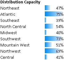
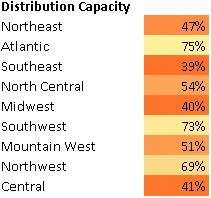
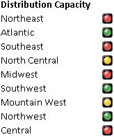
Note

Clicking the New Rule button in the Conditional Formatting Rules Manager displays the New Formatting Rule dialog box. The commands in the New Formatting Rule dialog box duplicate the options displayed when you click the Home tab's Conditional Formatting button.

After you create a rule, you can change the format applied if the rule is true by clicking the rule and then clicking the Edit Rule button to display the Edit Formatting Rule dialog box. In that dialog box, click the Format button to display the Format Cells dialog box. After you define your format, click OK.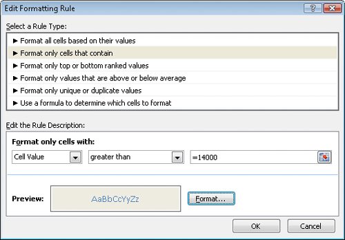

Important

Excel 2007 doesn't check to make sure that your conditions are logically consistent, so you need to be sure that you enter your conditions correctly.

Excel 2007 also enables you to create three new types of conditional formats: data bars, color scales, and icon sets. Data bars summarize the relative magnitude of values in a cell range by extending a band of color across the cell.

Color scales compare the relative magnitude of values in a cell range by applying colors from a two- or three-color set to your cells. The intensity of a cell's color reflects the value's tendency toward the top or bottom of the values in the range.

Icon sets are collections of three, four, or five images that Excel 2007 displays when certain rules are met.

When you click a color scale or icon set in the Conditional Formatting Rule Manager and then click the Edit Rule button, you can control when Excel 2007 applies a color or icon to your data.

Caution

Be sure to not include cells that contain summary formulas in your conditionally formatted ranges. The values, which could be much higher or lower than your regular cell data, could throw off your formatting comparisons.

In this exercise, you create a series of conditional formats to change the appearance of data in worksheet cells displaying the package volume and delivery exception rates of a regional distribution center.

USE the Dashboard workbook in the practice file folder for this topic. This practice file is located in the My Documents\Microsoft Press\Excel SBS\Appearance folder.

OPEN the Dashboard workbook.

1.	Select cells C4:C12.
2.	On the Home tab, in the Styles group, click Conditional Formatting. From the menu that appears, point to Color Scales, and then, in the top row of the palette that appears, click the second pattern from the left. Excel 2007 formats the selected range.
3.	Select cells F4:F12.
4.	On the Home tab, in the Styles group, click Conditional Formatting. From the menu that appears, point to Data Bars, and then click the light blue data bar format. Excel 2007 formats the selected range.
5.	Select cells I4:I12.
6.	On the Home tab, in the Styles group, click Conditional Formatting. From the menu that appears, point to Icon Sets, and then, in the left-hand column of the list of formats that appears, click the three traffic lights. Excel 2007 formats the selected cells.
7.	With the range I4:I12 still selected, on the Home tab, in the Styles group, click Conditional Formatting, and then click Manage Rules. The Conditional Formatting Rules Manager appears.
8.	Click the icon set rule and then click Edit Rule. The Edit Formatting Rule dialog box appears.
9.	Select the Reverse Icon Order check box. Excel 2007 reconfigures the rules so the red light icon is at the top and the green light icon is at the bottom.
10.	In the red light icon's row, click the Type field down arrow and then click Percent.
11.	In the red light icon's Value field, type 80.
12.	In the yellow light icon's row, click the Type field down arrow and then click Percent.
13.	In the yellow light icon Value field, type 67.
14.	Click OK twice to clear the Edit Formatting Rule dialog box and the Conditional Formatting Rules Manager. Excel 2007 formats the selected cell range.
15.	Click cell C15.
16.	On the Home tab, in the Styles group, click Conditional Formatting. From the menu that appears, point to Highlight Cells Rules and then click Less Than. The Less Than dialog box appears.
17.	In the left field, type 96%.
18.	Click the With field down arrow and then click Red text.
19.	Click OK. The Less Than dialog box disappears, and Excel 2007 displays the text in cell C15 in red.

CLOSE the Dashboard workbook.