Optimizing for Image Content

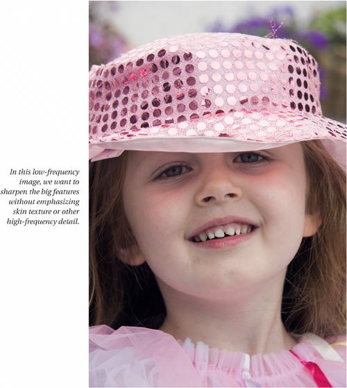
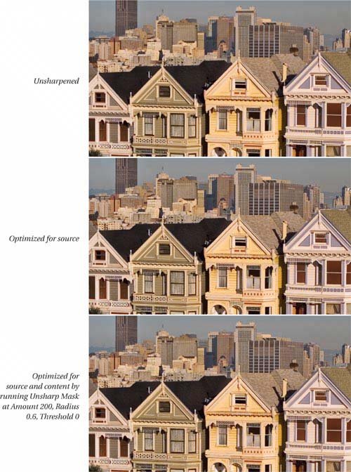
Once the source optimization is completed, the next step in the workflow is to optimize for image content. See "Sharpening and Image Content" in Chapter 2, Why Do We Sharpen? for a discussion of the differing requirements imposed by image content. In this section, I'll concentrate on the process.

For all image types, the process is the same. We start by creating a layer mask that protects the non-edges and exposes the edges to editing, we apply that layer mask to the sharpening layer we used to optimize for source, and then we apply additional sharpening to that masked layer. The control points are the degree of blurring applied to the mask, and the sharpening settings used.

In this section, I'll show you typical optimizations for a high-frequency image, a mid-frequency image, and a low-frequency image. For any given image source, I find that it works quite well to treat all images as either low-, mid-, or high-frequency, but if you want more nuanced manual treatments, you can make the mask blurring and layer sharpening adjustments by hand on each image, trading more control for more work.

Content Optimization, Low-Frequency

The image in Figure 5-22 contains mid-frequency and high-frequency components, but the general tendency is low-frequency: I want to sharpen the dominant features without emphasizing high-frequency detail like skin texture. I can accomplish this using the combination of a soft-edged mask and a fairly wide sharpening Radius.

Figure 5-22. A low-frequency image

The starting point is the sharpening layer used to optimize for the image source. It may seem a scary prospect to sharpen this layer again, but bear in mind that the combination of the layer's reduced opacity (66 percent), the effect of the Blend If sliders in forcing the sharpening into the midtones, and the effect of the layer mask attached to the sharpening layer all act together to make the sharpening quite mild.

Low-frequency Edge Mask

I've used several techniques in the past to create low-frequency edge masks, but the one that seems to work best in the greatest number of cases is to start out with a blurred copy. I make this by creating a layer using Option-Merge Visible, which I then blur with Gaussian Blursee Figure 5-23.

Figure 5-23. Creating a blurred layer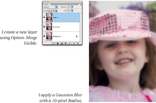

To create the mask channel, I use Calculations, blending the Red and Green channels with Pin Light blend, and making sure that the blurred layer is selected for both sourcessee Figure 5-24.

Figure 5-24. Creating the mask channel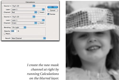

Running Find Edges, then Levels, followed by Image>Adjustments>Invert creates a soft-edged masksee Figure 5-25.

Figure 5-25. Making a soft edge mask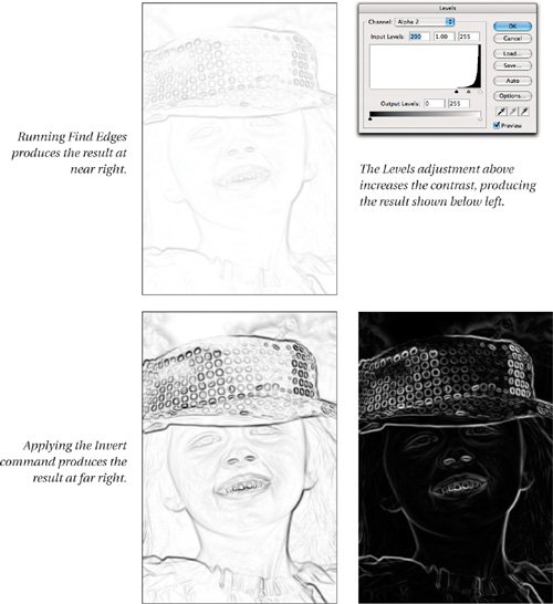

The mask is almost finished. The extreme tonal edit has introduced some posterization in the midtones, which I soften using a second Gaussian Blur with a Radius of 10 pixels. Gaussian Blur makes more tonal values available and hence reduces posterization, but it also reduces the contrast, so I finish off the mask channel with another, gentler Levels adjustmentsee Figure 5-26.

Figure 5-26. Fine-tuning the mask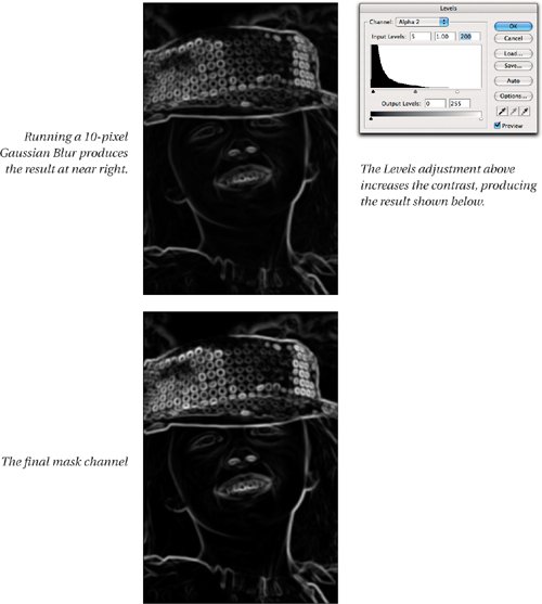

Loading the Mask

With the mask channel completed, I can now load it as a selection, and add it to the sharpening layer as a layer mask. Once I've done so, I can delete both the blurred layer and the alpha channel, since they've served their purpose, to keep the file size down. If I need to retrieve the alpha channel, I can do so by targeting the sharpening layerthe layer mask then appears in the Channels palette. Figure 5-27 shows the steps for adding the layer mask and deleting the layer and the alpha channel.

Figure 5-27. Loading the mask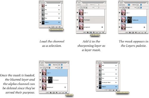

Final Sharpening for Content

With the mask in place, I can now apply the sharpening for content. Since I'm applying the sharpening to a masked layer with reduced opacity, I can apply strong sharpening and still obtain a very subtle result. Note that the proxy view in the Unsharp Mask filter ignores both the mask and the layer opacity, so it looks quite scary! Figure 5-28 shows the results of the final sharpening, with Unsharp Mask at Amount 180, Radius 3, Threshold 0.

Figure 5-28. Final sharpening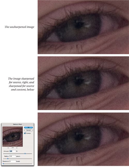

Notice that the final optimization for source and content has less sharpening than the image optimized for source. That's an intended effect of the layer mask. The initial optimization for source simply makes the content optimization more effectiveit's not designed as a global sharpen.

The variables in the content optimization are the values for the two rounds of Gaussian Blur, the first on the blurred layer, the second on the mask channel itself; and the settings for the final Unsharp Mask step. This example is an 8.2-megapixel digital capture. For smaller files, reduce the Radius settings slightly, and for larger ones, increase them. I'll discuss the numbers in more detail later in this chapter. First, to provide more context for that discussion, let's look at medium- and high-frequency images.

Content Optimization, Mid-Frequency

The optimization process for mid-frequency images is the same as for low-frequency ones: The only difference is the values used for the Gaussian Blurs and for the final sharpening. Again, we start with the sharpening layer created during the source optimization.

Figure 5-29 shows a mid-frequency image. It has low- and high-frequency components, but the dominant tendency I want to emphasize is the medium-frequency edges.

Figure 5-29. A mid-frequency image

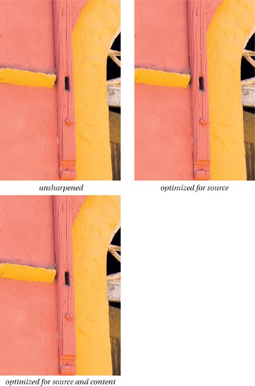
For this type of image, I use a much smaller Radius setting for the Gaussian Blur I apply to make the blurred layer, and an even smaller Radius setting for the Gaussian Blur applied to the mask. The reason for using a blurred layer is to influence the behavior of the Find Edges filter.

If I don't build the layer mask from a blurred layer, Find Edges creates very narrow edges that produce a sharp transition between sharpened and unsharpened pixels. I can mitigate this to some extent by blurring the mask itself, but for low- and mid-frequency images, working from a blurred layer is more effective. Figure 5-30 shows the stages involved in creating the edge mask for this image.

Figure 5-30. Creating the edge mask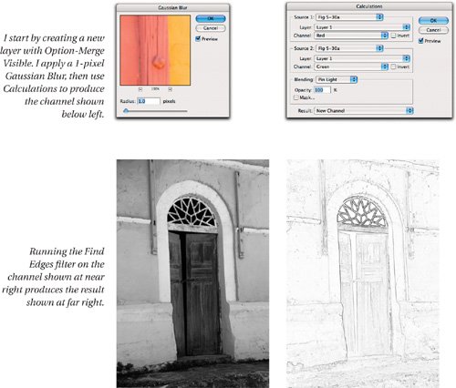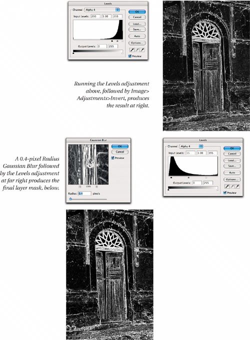

Once the mask channel is finalized, the procedure for adding it to the sharpening layer and deleting the blurred layer and the mask channel is identical to that for the low-frequency image. I can then apply the final sharpening for content by targeting the sharpening layer and running Unsharp Mask with Amount 200, Radius 0.8, Threshold 0. Figure 5-31 shows a detail from the image before and after optimization.

Figure 5-31. Mid-frequency optimization

Content Optimization, High-Frequency

The procedure for sharpening a high-frequency image for content differs from that for low- and mid-frequency images in that there's no need to create a blurred layer. Instead, we simply blur the mask channel after running Find Edges. On some images, the mask may need tonal editing, but I prefer to wait until the sharpening has been applied before making that decision. Figure 5-32 shows a high-frequency image with lots of fine detail.

Figure 5-32. A high-frequency image

Making the Mask

Creating the edge mask for this type of image is a simpler process than for low- or mid-frequency images. I use Calculations to create a new channel, but instead of creating a blurred layer from which to do so, I instead start with the sharpening layer used for source optimization. Once the new channel is created, I run Find Edges. I use Image>Adjustments>Invert to invert the channel, and run a small-radius (0.8-pixel) Gaussian Blur. Figure 5-33 shows the process.

Figure 5-33. Creating the edge mask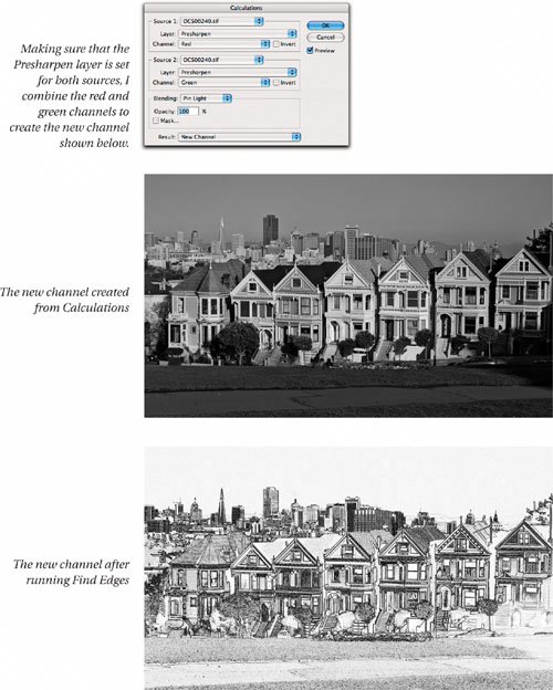

Since the mask generated by this method has been blurred only very lightly, it still covers a full tonal range, so the Levels edits required in the previous two techniques are unnecessary. I may edit the layer mask after sharpening has been applied, thoughsee "Post-Sharpening Control," later in this chapter.

Adding the layer mask uses the same technique as the previous optimizationsload the channel as a selection, target the sharpening layer, add the mask, then sharpen. Figure 5-34 shows the result of the sharpening.

Figure 5-34. Before and after sharpening

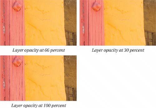
Post-Sharpening Control

Once the sharpening (and when appropriate, noise reduction) layers have been applied, you still have considerable control over the sharpening. The first level of control is the layer opacity of the sharpening layer. Creating the layer with an opacity of 66 percent means that you can increase or decrease the sharpening effect by adjusting the layer opacity up or down.

Figure 5-35 shows the effects of adjusting the layer opacity.

Figure 5-35. Sharpening layer opacity

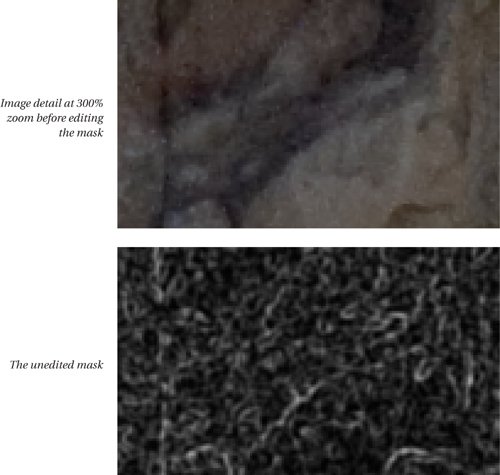
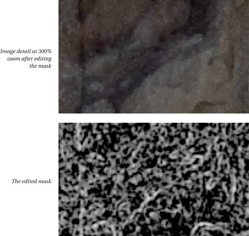
Finer control is offered by editing the layer mask. You can use any of Photoshop's tools to edit the layer mask, but the one I use most often is Levels.

Levels and the Layer Mask

Photoshop's Levels command offers an easy yet powerful way to edit the layer mask. Remember the basic rule of maskswhite reveals, black concealsso you can influence the sharpening in several ways by editing the sharpening layer mask. Figure 5-36 shows how each control in Levels affects the sharpening layer.

Figure 5-36. Levels and masks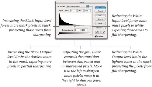

I rely heavily on presets for my sharpening because I process lots of images, and I find that the combination of the layer opacity and mask editing lets me tweak the sharpening to produce results that very similar to those I would have achieved doing the entire process by hand.

Figure 5-37 shows a typical layer mask edit with Levels.

Figure 5-37. Editing the mask with Levels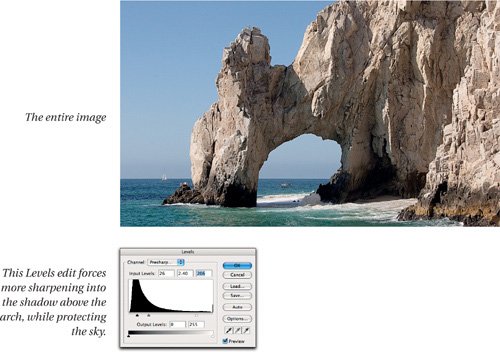

Simple Levels edits like the one shown in Figure 5-37 take care of the vast majority of fine-tuning requirements. In more extreme situations I may resort to Curves, for fine-tuning very specific tonal ranges of the mask.

If the mask starts to exhibit objectionable posterization (meaning that you see sharp transitions between sharpened and unsharpened pixels), Gaussian Blur can help by making more tones available. Gaussian Blur will also soften the mask, of course, but you can use the gray slider in Levels, or a Curves adjustment, to "choke" the softened edges back, if indeed that's what you want to do. Very subtle adjustments can be achieved this way.

Automating Content Sharpening

You can take the action described earlier for source sharpening and turn it into a complete presharpening routine. You'll need to make at least two separate actions, one for source sharpening that uses a blurred layer to make the mask, the other for source sharpening that calculates the mask layer directly from the presharpening layer. If you want to incorporate noise reduction too, you'll need to create separate actions with and without noise reduction.

Then you'll have to decide whether you want to create multiple actions with presets for different image sources and resolutions, or toggle the dialog boxes on for those steps where the numbers depend on the image.

A Complete Presharpening Action

Here is a procedure for creating an action that applies sharpening for both source and content in a single routine. In this example, I'll use the values that are appropriate for a mid-frequency 8-megapixel capture, but I'll also point out the steps where you'd vary the numbers for other image types.

I start with the action previously described for automating source optimization. To extend it, select the last action stepUnsharp Maskand click the Record button in the Actions palette. It's a good idea to open a suitable image and run the source optimization action on it before starting to extend the actionsee Figure 5-38.

Figure 5-38. Extending the source optimization action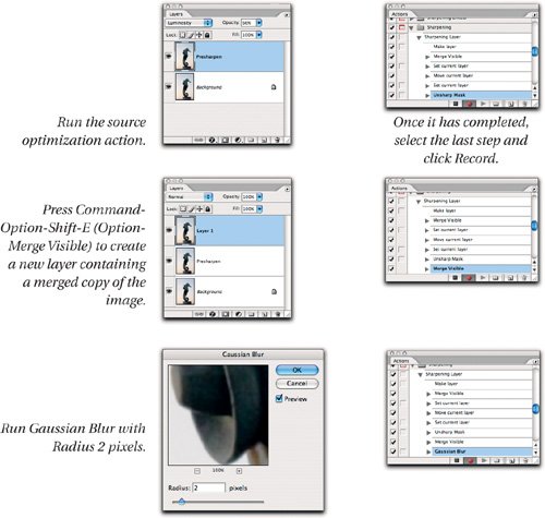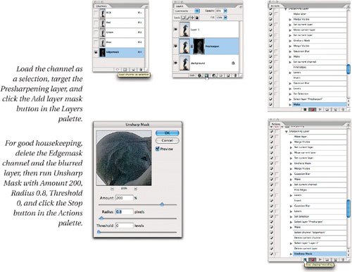

To exercise manual control while you're running the action, turn on the dialog boxes for the steps shown in Figure 5-39.

Figure 5-39. Actions with manual control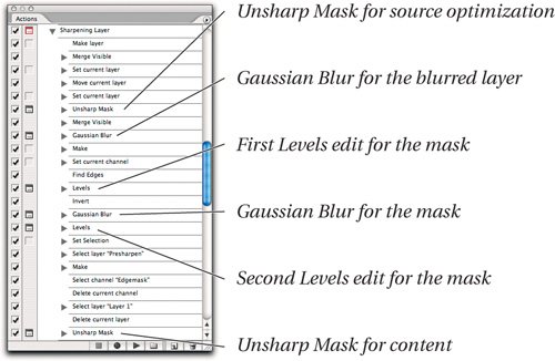

Controlling File Size

Sharpening and noise reduction layers and masks add significantly to the size of the file. A single sharpening layer doubles the size of the file, and each extra channel or layer mask adds one-third of the original file size. So file sizes can balloon quite quickly.

Of course, the only way to retain complete control over the sharpening is to keep the layers intact, and take the hit on file size. Other sensible strategies are:

• Once you've tweaked the sharpening to your satisfaction, archive the layered file and continue to work on a flattened copy.

• Once you've tweaked the sharpening to your satisfaction, simply flatten the image.

• To retain some degree of control over the sharpening, create a new layer using Option-Merge Visible, then delete the sharpening layers and masks. Note that the merged layer will be a Normal blend layer with 100 percent opacity, so you won't be able to reduce the sharpening. You can work around this by increasing the opacity of the sharpening layer to 100 percent before creating the merged layer, then you can reduce the opacity of the merged layer to the strength you preferred.