6.2 Basic definitions

---

6.2 Basic definitions

A stochastic process involves the representation of a family of random variables. A random variable is represented as a function on a variable, f(x), which approximates a number with the result of some experiment. The variable X is one possible value from a family of variables, from a sample space represented as Ω. For example, for a toss of a coin the entire sample space is Ω = {heads, tails}, and the random variable X may equal the mapping x = {1,0}, representing the functional mapping of the event set {heads, tails} to the event random variable mapping set {1,0}. (SeeTable 6.1.)

Table 6.1: Functional Mapping

Events	=	Heads	Tails
		↓	↓
X	=	0	1

A stochastic process is represented or described as a family of random variables, denoted X(t), where one value of the random variable X exists for each value of t. The random variable, X, has a set of possible values defined by the state space, X(t), for the random variable X, with values selected by the parameter set, T (sometimes called the index set), whose values are drawn from a subset of the total index set T.

As with random variables, stochastic processes are classified as being continuous or discrete. Stochastic processes can have either discrete or continuous state spaces as well as discrete or continuous index sets. For example, the number of commands, X(t), received by a timesharing computer system during some time interval (0,t) can be represented as having a continuous index parameter and a discrete state space. A second example could be the number of students attending the tenth lecture of a course. This can be represented as having a discrete index set and a discrete state space. In general, if the number of states in the state space is finite, then the stochastic process has a discrete state space. Likewise, if the index set for the state space is finite and counting, then the index set is also discrete. For continuous systems, the number of possible values for the variables are not discrete (i.e., real valued). For the index set to be continuous, the set of possible values must be real and can approach infinite.

One important form of stochastic process is the counting process. A counting stochastic process is one where we wish to count the number of events that occur in some time interval, represented as N(t), where N is drawn from the discrete set of counting positive integers from the set {0,1,2,3,...}. In addition, the index set for such a counting stochastic process is drawn from the continuous space of time, where time is from some reference point {t ≥ 0}. The requirement for this stochastic process is that for the value of the index set 0, the random variable N(0) = 0. For values of t < 0, the value of N(t) is undefined. This implies that the values of N(t) only exist for values of the index set above 0, and the values of N(t) for all ranges of t above 0 are positive nonnegative values. A second property for a counting stochastic process deals with the relationship discrete values drawn from the state space have with each other. For any two values of the index set—for example, indexes s and t, where s < t—the values of the random variables must have the relationship X(s) ≤ X(t). Finally, if we look over some interval of values for the index set—for example, values s and t— N(t) - N(s) represents the number of events from our represented events that have occurred by time t after time s and bounded by t.

When discussing stochastic processes, it is often important to be able to determine the order of a function, such that we can focus on the dominant component. One way of doing this is to use notation from computer science and analysis of algorithms. The definition of the "order" of computa- tion for an algorithm is often referred to as the order of a function. Two common ones are little-oh, written o(h), and big-oh, written O(h), where h indicates the variable of the function. Little oh describes the order or size of a function as the value of the function, when divided by the value of h, approaches the limiting value of o, as it approaches 0. This is depicted as:

(6.1) 

If a function of h, when divided by h, does not result in 0, then the function is not o (h). If it does approach 0 as the limit is approached, then the function is o (h). For example:

(6.2)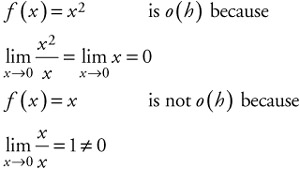 

This concept of the order of a function can be used in understanding stochastic processes and in simplifying their analysis, as will be shown. For example, suppose x is an exponential random variable with parameter λ and is described by the following probability function:

(6.3) 

We may wish to determine what the probability is that x is less than t+ h given that it is greater than t. (See Figure 6.1.)

Figure 6.1: Stochastic process for P[x≤t+h|x>t].

(6.4) 

Jumping ahead and applying a concept not yet described—that of the Markov property of exponential distributions—we can show that:

(6.5)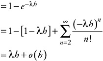 

This indicates that the function order is o(h).

Another important property is that of independent and stationary increments. A stochastic process has independent increments if events in the sample space {x(t), t ≥ o}, occurring in nonoverlapping intervals, do not have the same value. For example, with regard to Figure 6.2, x(b1) -x(a1) ≠ x(b2) - x(a2).

Figure 6.2: Independent stochastic processes.

A stochastic process has a stationary increment if the values of a random variable over similar ranges are equivalent. For example, if over two intervals x(t), x(s) and x(t+ h), x(s + h), the value for x(t+ h) -x (s + h) has the same distribution as x(t) - x(s) for all values of h > 0, then the stochastic process has stationary increments. (See Figure 6.3.)

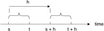
Figure 6.3: Stationary stochastic processes.

Another way of looking at this definition is that if x(t) - x(s) = x(t + h) - x(s + h), then this stochastic process has stationary increments.

As an example, we assume N(t) is the number of phone calls handled by a certain central office between midnight and some time, t, on a workday (Figure 6.4).

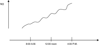
Figure 6.4: Example phone call volume.

This process can be looked at as possessing independent increments, not stationary increments. If we look at two values for time, 8:00 A.M. and 12:00 noon, the values from 8:00 A.M. to 10:00 A.M. and from 12:00 noon to 2:00 P.M. do not show the same value for the variable N(t). Therefore, this stochastic process does not have stationary intervals but does have independent increments.

These concepts of discrete and continuous state space and index set, along with the concepts of independent and stationary increments, can be used to further understand the properties of various systems—for example, if we look at another stochastic process: tossing of a fair coin. We can describe one such stochastic process as counting the number of heads flipped during n flips of a fair coin. Such a stochastic process is referred to as a Bernoulli process. If we let X₁, X₂, X₃, ... be independent identically distributed Bernoulli random variables, the property for each value of x is:

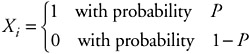
The value of 1 represents a successful outcome (e.g., flipping a head), and 0 represents the failure of flipping a head.

(6.6) 

Therefore, S_n is a Bernoulli process (discrete parameter, discrete state).

For each n, S_n has a binomial distribution:

(6.7)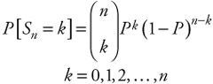 

Starting at any point within the sample space, the number of trials, y, before the next success has the geometric distribution with the probability:

(6.8) 

---