15.3 Simulation modeling of local area networks

---

15.3 Simulation modeling of local area networks

15.3.1 Computer networks (the model)

A computer network can be considered to be any interconnection of an assembly of computing elements (systems, terminals, etc.) together with communications facilities that provide intra- and internetwork communications.

These networks range in organization from two processors sharing a memory to large numbers of relatively independent computers connected over geographically long distances. (The computing elements themselves may be networks, in which case it is possible to have recursive systems of networks ad infinitum.) The basic attributes of a network that distinguish its architecture include its topology or overall organization, composition, size, channel type and utilization strategy, and control mechanism.

Using the nomenclature and taxonomy discussed for computer interconnection structures, a particular system can be characterized by its transfer strategy (direct or indirect), transfer control mechanism (centralized or decentralized), and its transfer path structure (dedicated or shared). Various network topologies, such as ring, bus, and star, are seen as embodiments of unique combinations of these characteristics (see Figure 15.11).

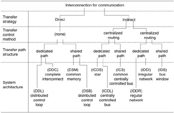
Figure 15.11: Taxonomy of computer interconnection structures.

Network composition can be either heterogeneous or homogeneous, depending on either the similarity of the nodes or the attached computing elements. Network size generally refers to the number of nodes or computing elements. With respect to its communications channels, a network may be homogeneous or it may employ a variety of media. Overall network control or management is usually either highly centralized or completely distributed. If the hardware used for passing line control from one device to another is largely concentrated in one location, it is referred to as centralized control. The location of the hardware could be within one of the devices that is connected to the network, or it could be a separate hardware unit. If the control logic is largely distributed throughout the different devices connected to the network, it is called decentralized control.

Implementation-independent issues that are dependent on system attributes are modularity, connection flexibility, failure effect, failure reconfiguration, bottleneck, and logical complexity. A subset of all possible computer systems is that of local computer networks (LCNs). Although no standard definition of the term exists, an LCN is generally regarded as being a network so structured as to combine the resource sharing of remote networking and the parallelism of multiprocessing. A usually valid criterion for establishing a network as an LCN is that its internodal distances are in the range of 0.1 to 10 km with a transfer rate of 1 to 100 Mbps.

Bus-structured LCN

The range of systems to be studied will be confined to what is known in the LCN taxonomy as category 3 bus-structured systems (Figure 15.12). As opposed to such point-to-point media technologies as circuit and message switching, a bus-structured system consists of a set of shared lines that can be used by only one unit at a time. This implies the need for bus-control schemes to avoid inevitable bus-use conflicts.

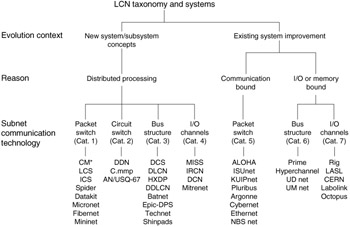
Figure 15.12: Local computer networks taxonomy.

Network components

As a first step in developing a general LCN simulation, the network model illustrated in Figure 15.13 is established. A network consists of an arbitrary number of interconnected network nodes. Each node consists of one or more host computing elements or processors connected to an independent front-end processor termed an interface unit (IU).

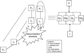
Figure 15.13: Generalized distributed computer network.

The hosts are the producers and consumers of all messages, and they represent independent systems, terminals, gateways to other networks, and other such instances of computing elements. The IUs handle all nodal and network communication functions, such as message handling, flow control, and system reconfiguration. The lines represent the physical transmission media that interconnect the nodes. The IUs, together with the line interconnection structure, comprise the communication subnetwork.

The model in Figure 15.13 isolates the major hardware units involved in the transfer of information between processes in different hosts. At this level no distinction is made between instances of messages such as data blocks and acknowledgments. In order to develop and refine the model, the major elements, structures, and activities must be further defined.

Host processors

Host or processor components generally include computation and control elements, various levels of memory, and input and output peripherals. As far as the system is concerned, each processor's behavior can be considered to be reflected in appropriate distribution functions that describe the rate at which the processor produces and consumes interprocessor messages. These functions reflect a given processor's inherent processing power and loading based on processor parameters, exogenous communication levels, and internetwork communications.

Queues

Queues are shared memory buffer structures through which information transfer between a processor and its IU takes place. For each node there will be an output (line) queue for messages awaiting transmission as well as one or more input (message) queues containing unprocessed receptions. The queue memory area may be located in the processor or in the IU depending on the implementation. Functionally, both are equivalent.

Associated with queues are control variables, which are maintained and monitored by both the processors and IUs to provide for the simultaneous and asynchronous access of the queues. The most common types are linear, circular, and linked queues. Linear queues (buffers) are used when the extent of a message is known and the buffer structure can be allocated in advance. The use of circular buffers is appropriate if several messages of undetermined length are to be buffered before one of them is processed. A pool of chained queues is used if the message sizes and arrival times vary over wide ranges that cannot be predicted in advance and the messages are not removed in order of their arrival.

Messages are deposited (written) into and withdrawn (read) from queues using various strategies such as FIFO (first-in, first-out), LIFO (last-in, first-out), and longest message first.

Queue access is controlled in order to prevent writing into a full queue, reading from an empty queue, and reading information as it is being written.

Interface units

Insofar as its role in the network is concerned, the interface unit is the most complex unit with respect to both hardware and software. The basic function of the IU is to enable its processor to communicate with others in the network as well as to contribute to overall network functioning. This involves system (re)initialization, flow control, error detection, and management.

When the IU detects that its processor has a message to send, it formats the message for transmission and becomes a contender for exclusive use of the communications channels. Upon allocation of control, the controller transmits the message and, depending on the implementation, may await a response from the destination processor.

Upon completion of resource (bus) utilization, the IU must be able to pass control to the next candidate according to the allocation scheme. If there is an IU failure, the other IUs must be able to substitute for it insofar as its network control responsibilities are concerned.

Communication lines

The lines are the physical connections between network nodes over which control and data transmissions travel. Common equivalent terms are channel and circuit. A particular circuit is either uni- or bi-directional (by nature and/or use) and supports continuous transmissions provided by analog or digital techniques.

Circuits are supported using a variety of media, such as coaxial cables, twisted pairs, fiber optics, microwave links, laser links, and so on. For the purposes of the simulation it is not necessary to be concerned about these low-level characteristics except as they are represented by a set of channel characteristics: the maximum data rate, delay and error parameters, and directional limitations.

It is also useful to consider setup characteristics if a point-to-point circuit is not always dedicated to a network. These setup characteristics may include the signaling mechanism and delay, circuit setup delay, and the delay for breaking the circuit. In the systems that will be examined later in the chapter, setup characteristics will not be a factor.

Maximum data rates vary from 50 Kbps (twisted pair) up to 150 Mbps (optical cables). This rate represents the raw transmission capability of the line and is not the same as the net rate at which information is transferred. There is always an overhead. Various factors, such as logic failures, electronic interference, and physical damage, give rise to transmission degradations ranging from single-bit errors to total line failure. Depending on the type of line used, typical error rates vary from 1 in 10,000 to 1 in 10,000,000 bits transmitted.

Interconnection structures

Various network aspects, such as scheduling, message routing, and reconfiguration, are fundamentally related to a network's physical interconnection structure. For example, eligibility for bus control may be dependent on position, the time for a message transfer may be dependent on the location of the processors involved, or a network's continued functioning may be contingent upon the existence of a redundant link. This structure may be represented by a topological organization of the three hardware archetypes-nodes, paths, and switches-that are involved in the transfer of information between processes at different nodes.

These transfers are called message transmissions and do not distinguish between instances of messages, such as data blocks, service requests, semaphores, and so on. Likewise, in restricting consideration to structural issues it is unnecessary to distinguish between a computing element and its interface. They are lumped together as the entity node. The switching elements affect the routing or the destination in some way.

Figure 15.14 shows a general model of an interconnected system. For simplicity, the class of systems with only one switch is represented.

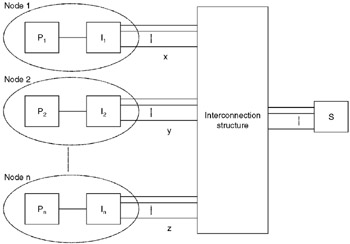
Figure 15.14: General interconnection model.

Associated with each node and switch are a number of paths or links. Each node can connect to the rest of the network through one, two, or multiple links corresponding, respectively, to a bus system, a ring or loop structure, or a fully interconnected network with direct links between each pair of nodes. Figure 15.15 shows specific examples of interconnection structures.

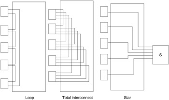
Figure 15.15: Examples of interconnection structures.

These diagrams suggest that the interconnection structure can be represented by or implied in tables and/or algorithms that will enable the determination of such things as the next eligible node for resource utilization, internodal lengths, reconfiguration parameters, and optimal paths. A complete representation might be underutilized in the present simulation effort but would provide for increased sophistication in the future.

If the node is resolved into its components (i.e., the computing element and IU), it can be seen that the model can represent the interconnection aspects of the various control schemes possible for distributed networks. Since no assumption is made about the nature of the components of a node or of its communications with the rest of the network, it is possible for a particular node to represent a centralized controller dedicated solely to network management instead of a host processor in the usual sense.

15.3.2 Protocols

Network activities occur in a potentially hostile environment because of such factors as nonhomogeneous components, limited bandwidth, delay, unreliable transmissions, and competition for resources. In order to provide for the orderly coordination and control of activities, formal communication conventions or protocols have been developed that encompass the electrical, mechanical, and functional characteristics of networks.

These protocols are almost always complex, multilayered structures corresponding to the layered physical and functional structure of networks. Each lower layer is functionally independent and entirely transparent to all higher-level layers. However, in order to function, all higher-level layers depend on the correct operation of the lower levels.

Every time one protocol communicates by means of a protocol at a lower level, the lower-level protocol accepts all the data and control information of the higher-level protocol and then performs a number of functions upon it. In most cases, the lower-level protocol takes all the data and control information, treats it uniformly as data, and adds on its own envelope of control information. It is in the format of messages flowing through a network that the concept of a protocol hierarchy is most evident. The format of transmitted messages shows clearly the layering of functions, just as a nesting of parentheses in a mathematical expression or in a programming language statement does.

Among the functions provided by protocols are circuit establishment and maintenance, resource management, message control, and error detection and correction. Performance of these functions provided by protocols are circuit establishment and maintenance, resource management, message control, and error detection and correction.

Performance of these functions introduces delays in data transmission and requires adding headers and other housekeeping data fields to messages as well as requiring acknowledgment of correct reception or retransmission in case of errors. This reduces the useful data rate of a network. These overhead aspects of message transfer transmission are taken into account in a measure of the efficiency of the protocols. In general, a protocol is simply the set of mutually agreed upon conventions for handling the exchange of information between computing elements. Although these elements could be circuits, modems, terminals, concentrators, hosts, processors, or people, the view taken in this section is restricted to hosts and processors embedded within other equipment.

The crux of maintaining a viable distributed environment lies in accepting the inherent unreliability of the message mechanism and to design processes to cope with it. In earlier systems, protocols were designed in ad hoc fashion. Typically, these protocols were application specific and implemented as such. All recent protocol work has been moving in the direction of a hierarchical, multilayered structure, with the implementation details of each layer transparent to all other layers and hierarchies.

Although there is no universal agreement on the names and numbers of protocol layers, a widely accepted standard is the International Organization for Standardization, (ISO), Open System Interconnect (OSI) model, which is shown in Figure 15.16. Using this organization, level 1 (physical layer) protocols include RS-232 and X.21 line-control standards, Manchester II encoding, encryption, link utilization time monitoring and control, transmission rate control, and synchronization.

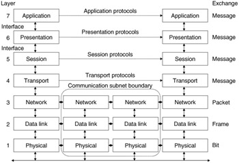
Figure 15.16: ISO OSI model.

Level 2 (data link) provides for the reliable interchange of data between nodes connected by a physical data link. Functions include provision of data transparency (i.e., providing means to distinguish between data and control bits in a transmission); contention monitoring and resolution; the establishment, maintenance, and termination of interactions (transactions); error detection and correction; and nodal failure recovery.

A description of the operational aspects of the general network is best presented in the context of the previously defined protocol structure, since all possible network events and activities, intentional and otherwise, must be managed under this structure. The protocol structure also implies the underlying structures and functional mechanisms that support network operation.

Before any control or data communications can be conducted, the actual means of signaling and bit transmission across a physical medium must be provided. Physical links must be established in accordance with the specified network topology and line parameters.

Frequently, an encoding scheme such as Manchester II is used on this level to provide for synchronization and error detection. In the Manchester II scheme each of the original data bits is transformed into two transmission bits in such a way that it is impossible to get three consecutive identical bits in the encoded message. This implies that the message receiver can detect errors by watching for this occurrence. Also, this encoding can be selectively disabled to provide unique, invalid waveforms that can be used as synchronization signals.

Given the physical layer service capability to exchange signals across the physical medium, the data link layer is implemented to provide the capability of reliably exchanging a logical sequence of messages across the physical link. The fundamental functions of the layer include the provision of data transparency, message handling, line management, and error control. Since, in the original case, data and control information pass along the same line during a transmission, certain techniques must be provided to distinguish between the two. This is done by assigning control meanings to certain bit patterns that are prevented from occurring in the data stream through the use of such techniques as bit and byte stuffing and the previously described Manchester scheme. In this way, control sequences can be used to delimit the beginning and end of asynchronously transmitted, variable-length messages. Common expressions for such sequences include BOM, EOM, and flag.

The elementary unit of data transmission is usually the word. The number of data words in a message is generally variable up to some maximum message length (MML), and a parity bit is usually appended to data and control words. Each message must include addressing information whenever the sender and receiver are not directly connected. Addresses may be physical, in which case each node has a unique address, or they may be logical, in which case each node has associated with it one or more coded sequences representing functional entities. A particular logical address may be associated with an arbitrary number of physical nodes, thus providing for single, multiple, or broadcast addressing. Address information may be contained in the data portion of a message or it may be part of the control information.

Each transaction may be considered to be either a bilateral or a unilateral process, depending upon whether or not the sending process requires a response from the destination concerning the success of the transmission. In the systems in which a choice can be made between these alternatives, the message must contain information about this choice. Response types include but are not limited to the following:

• NO REPLY REQUESTED-In the case of a message being sent to a process where multiple copies exist, the issuance of an acknowledgment is undesirable because collisions would result.

• STATUS REQUESTED-Information regarding the success or failure of the transmission is requested.

• LOOPBACK REQUESTED-Loopback is the situation in which a destination node is also the source node.

15.3.3 Transmission error detection

In order to ensure that a transmission is occurring without error, it is necessary for the link control level to include a set of conventions between the sender and receiver for detecting and correcting errors.

There are many possible methods for error control over a transmission link. Two general types of error control are forward error control and feedback error control. The most practical and prevalent method is feedback control.

The simplest form of detection is a parity check on each transmitted character. This is often called a vertical redundancy check, and it is used to provide protection against single bit errors within characters. A horizontal or longitudinal redundancy check (LRC) provides for a check across an entire message. This is done by computing a parity bit for each bit position of all the characters in the message. The most powerful form of check is the cyclic redundancy code check (CRC), which is a more comprehensive algebraic process capable of detecting large numbers of bits with errors.

There is a possibility that a message or response does not even arrive at its destination, irrespective of whether the information is good or bad. This can result from either a physical failure, such as the failure of the link or of the destination node, or a logical failure, such as the use of an incorrect destination name.

These possibilities can be detected by providing a time-out mechanism, which will cause a message to be retransmitted if, after an agreed upon delay (the response time-out), an acknowledgment has not been received. Many systems rely solely on the positive acknowledgment and time-out convention and do not employ a negative acknowledgment.

When multiple devices are sharing a bus, there must be some method by which a particular unit requests and obtains control of the bus and is allowed to transmit data over it. The major problem in this area is the resolution of inevitable bus request conflicts through the use of arbitration and scheduling schemes so that only one unit obtains the bus at a given time. Mechanisms must also be provided for system reinitialization and adjustment in the cases of system startup, nodal addition and removal, line failures, and spurious transmissions in the system.

In all systems collisions can occur when more than one control or data transmission simultaneously occurs. This may be caused by the use of random number techniques to generate allocation sequence numbers upon a node entering the system at startup or some later time, or it may be caused by a message with multiple destinations improperly asking for acknowledgment. Collisions are usually handled by the temporary or permanent removal of involved nodes or the retransmission of legitimate messages.

A limit is often imposed on line use time to prevent a node from monopolizing the bus, either intentionally or because of nodal failure. This condition may be prevented by placing a limit on the maximum message size and/or monitoring line use to determine when a node is maintaining an active transmission state beyond that required to send the largest allowed message.

This monitoring capability is achieved through the use of a loud-mouth timer, which is activated upon nodal allocation and provides an interrupt signal (or causes a collision) if allowed to run out. The usual outcome is the removal of power from the transmitter circuitry, either temporarily or permanently, and the informing of the host processor, when possible, of this condition.

When talking about control, it is important to keep in mind that this is not usually associated with a specific physical device or location but is rather a functional entity distributed (replicated) throughout the network.

15.3.4 Events

In order to precisely simulate the operational behavior of networks a more formal and quantitative analytical approach must be taken. In order to do this, the following concepts must be introduced. All actions and activities, intentional and otherwise, that can occur in system operation can be classified as events. An event is defined as any occurrence, regardless of its duration. Events have a number of characteristics, including the following:

• An event has a beginning, an end, and a duration.

• An event can be simple or complex. A simple event is one that cannot or, for the purposes of the simulation, need not be reduced into a simpler sequence of occurrences. Conversely, a complex event is one that consists of simpler events.

• An event may be a random occurrence or of a stochastic nature, or it may be the deterministic result (effect) of an identifiable cause.

• An event has a certain pattern of occurrence (e.g., periodic, aperiodic, synchronous, asynchronous, etc.).

• Events belong to classes. The significance of an event class is that each member has the same effect as each other in a particular context. For example, in certain systems the corruption of a message by noise is equivalent in effect to the incorrect specification of a destination name-both will result in a response time-out and a retransmission. Thus, these two events would be of the same class.

• Events may be concurrent or disjointed (sequential). Events that coincide or overlap in time are concurrent; otherwise, they are disjointed. The concept of effective concurrency is introduced here. Sequential program structures are considered effectively concurrent if they can successfully represent or model events that are actually concurrent.

An example would be the action of processors requesting services. While this is an asynchronous, unpredictable event(s) concurrent with channel utilization by a particular node, these two aspects of system behavior utilization and contention can be effectively separated, since (except in the case of interrupts) the request will not be acted upon until utilization is complete. As long as a record of the duration of utilization is available, an effective history of nodal requests can be generated just prior to contention resolution by the control module of the simulation program.

Following is a list of basic events that may be found to occur in the operation of various LCNs. All system behavior can be ultimately reduced to sequences of these simple events. Events are listed under the component in which they occur.

Processor

• Production. This is the generation of a message by a host computing element. Parameters associated with this event are production time, message size, destination(s).

• Queue inquiry. The determination by the processor of the state of an input or output queue before reading from or writing to it, respectively.

• Output message disposition. Depending upon the buffer availability strategy, a generated message may be queued normally, it may be written over exiting queued data, it may be held by the processor until it can be queued, or it may be dumped.

• Consumption (read message). This is the reading of a message in the input queue by the host computing element. Assuming a message is available in the input queue, it can be immediately consumed. Consumption with respect to a queue is similar to production.

• Node. It is convenient to associate the following events with the entity node rather than either the computing element or the IU.

• Addition. A node is considered added to the circuit when it informs the network that it wishes to be integrated into the system. This may occur upon initial power-up of the node or upon failure recovery.

• Integration. This is when the node actually becomes a functional part of the network.

• Failure. This is the failure of a node as a functional member of the network.

Interface unit

• Queue inquiry. This is analogous to the processor event.

• Read message. The IU obtains message from an output queue.

• Preprocess message. This is the formatting or packing of a message for transmission. It is to be distinguished from the formatting that is done by the processor.

• Request. The IU notifies the network that it wishes to use the bus. This may or may not involve the transmission of a control signal.

• Connection. This is the actual acquisition of the channel for utilization.

• (Re)transmission. This is the moment when the first word of a message is placed on the bus or, in the event of a message train, as in a ring structure, the first word of the first message.

• Response time-out activation. In systems in which a response to a message transmission is required within a certain amount of time, a response timer is activated at some point during transmission.

• Detection (identification). This is the detection by an IU of a message addressed to it.

• Reception. This is the moment when the complete message has been received, processing on it has been completed, and it is ready to be queued. This may also be considered queue inquiry time as well as response transmission time.

• Write message. This is when a received message is placed in the input queue.

• Response reception. This is when the message source receives information from the destination regarding the transmission.

• Delete message. This is the deletion of a message from an output queue following a successful transmission.

• Relinquish. Upon completion of utilization, the IU signals that reallocation is to occur.

Using these concepts, overall system activity or flow can be represented by the following sequence of complex events:

• NODAL ACTIVITY → CONTROL/ARBITRATION → UTILIZATION

This simple structure is possible because the concept of effective concurrency is valid in the case of global bus systems.

Nodal Activity

Nodal activity simulates the behavior of all nodes and interface units during the utilization period of a particular node. During this period nodal activity includes the following:

• The production and consumption of messages

• Queue activity

• IU background processing

• Addition and removal of nodes from the network

Control

Control may be a number of possible sequences depending on circumstances in which control is activated.

Utilization

The utilization event encompasses all activity associated with a node's utilization of the bus for the transmission of a message. Utilization begins with being connected to the bus and it terminates either gracefully, in the case of a successful transaction followed by a control output, or unintentionally, as the result of intervention by control because of a protocol violation (message too long, no reallocation signal transmitted, etc.).

15.3.5 The LAN simulator model structure

Based on the previous discussion of LAN structure and events, we can typify a LAN as consisting of three major hardware classes: host machines, interface units, and communications links. Additionally, these hardware classes possess varying levels of software and functionality.

The link level is concerned with the management and performance of bit-level physical transfers. This includes timing and control as well as mechanical and electrical interface. The interface units provide the main services to bring the simple communications media and protocols up to a true network. This component and its services must provide for node-to-node, host-to-node, and end-to-end protocols. This includes error detection and correction, media acquisition and control, routing, flow control, message formatting, network transparency, maintenance of connections, and other services. The host class of device provides the LAN with end-user sites that require remote services from other hosts. The services provided at this level are host-to-node interface, host-to-host protocols, and resource-sharing protocols. Implemented at this level of a LAN would be user-visible services, such as a distributed operating system, a distributed database management system, mail services, and many others. A model of this structure implies a minimum of a component for each of these items. Therefore, the simulator must have components of sufficient generality and flexibility to model these components and provide for analysis. Figure 15.17 depicts these basic components and the necessary simulation components to measure the performance and operations of a simulation. Using this structure, it can be seen that the simulator consists of a modular structure with components that can be turned to the modeling of specific LAN nuances. The physical and logical characteristics peculiar to each system design are contained in independent software routines and/or data tables. The high-level design of the LAN model shows the need for the following functions:

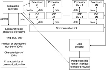
Figure 15.17: Basic components of a simulation model.

• A simulation controller, which will be responsible for the coordination and timely operation of the remaining software modules. This function will initialize the system architecture and distributed computing techniques in accordance with user input data, schedule events, calculate system state, maintain the common timetables, and initiate the processing of the other software routines as dictated by the particular logical and physical configuration.

• A system processor routine, which will be capable of simulating the time-dependent activity (data in, data out, processing time) of each proposed computing mode.

• An interface processing routine, which will be capable of simulating the activity (time delays, message handling, priority determination, addressing technique, resource allocation, etc.) of each proposed front-end processor as required by the particular logical and physical characteristics.

• A communications link routine, which will be capable of simulating the timing delays and the data and control transfer characteristics of the proposed transmission medium.

• A data collection routine, which will be responsible for collecting, formatting, and collating the requisite system evaluation parameters.

Data items collected will include, but will not be limited to, a minimum, maximum, and average of the following:

• Time to transmit message from A to B

• Message wait time

• Number of messages in the queue or system

• Message size

• Bus utilization

• Interface unit timing (as previously presented)

It will also include a postprocessing routine, which will be responsible for presenting the data in human-readable forms (graphs, plots, tables, etc.).

15.3.6 LAN simulator overview

This simulator was developed to provide a flexible research, development, and analysis tool for local area network architectures. The tool has been used to aid in the selection, development, and evaluation of local area network architectures that support large, distributed, real-time command control and communications (C3) environments.

The simulator was designed with the intention of comparing a wide range of possible distributed C3 configurations. This capability was achieved by providing the following:

1. A modular structure, which allows the model to be adapted to suit a variety of system specifications

2. A standard driving routine, which mimics the communications within a C3 system

3. A standard routine, which analyzes the distributed system on the basis of detailed evaluation criteria

Such a design allows for the implementation, testing, and evaluation of new strategies for improving system performance with little effort.

15.3.7 Next event simulation

The modeling technique used in the LAN software simulation is called next event simulation. Next event simulation views the world as a sequence of events rather than a continuum. If a department store checkout line is simulated in next event simulation, the process of checking out would be viewed as the following sequence: (1) a customer enters the checkout line, (2) the customer starts checkout, (3) the customer completes checkout. Between these events the customer is performing other activities, but these are unimportant if we are simply interested in the length of the waiting time.

The view of time taken by next event simulation is important in understanding the design and implementation of the LAN simulation. Time in next event simulation is viewed as a means of sequencing events and calculating time-related statistics. Events one hour or one second in the future are treated identically. Simulation is achieved by creating a file that contains future events along with the time of their occurrence. A simple loop program scans this file and selects the event with the lowest time. At that time, an internal memory location, which contains the simulated time, is updated to the occurrence time of the event. After the event occurs, mathematical calculations or logical operations can be performed to schedule other dependent events. In the checkout line example, this means that when checkout begins, the end of the checkout event is scheduled. In this way, the simulation proceeds from event to event and time constantly progresses.

The random or stochastic nature of scheduled events gives the simulation the characteristics of a real system. In the checkout line example, the time taken to serve a customer is not a constant; it may be one minute or ten minutes. The service time is also randomly distributed. That is to say, the service time of previous customers does not have any effect on future customers. The service times usually fall into a pattern; that is, it may be highly likely that a service time is 5 minutes but relatively unlikely to be 20 minutes. The likelihood of certain service times can be described by theoretical patterns called distributions. These distributions can be used to generate service times or arrival patterns that resemble those occurring in real systems.

15.3.8 LAN model implementation

The LAN simulator is a general-purpose simulation package used for modeling a wide range of local area network architectures. Its basic structure is shown in Figure 15.18 and consists of the following five major components:

1. Arrival module. The arrival module is concerned with generating the messages to be communicated and places them in an interface unit queue. It must also handle the queue overflow problem and the possibility of a processor being unavailable.

2. Arbitrator module. The arbitrator module is concerned with the determination of which interface unit will communicate over the link next, based on the policy of the communications link control in place.

3. Use module. The use module is concerned with the modeling of the passage of messages from source to sink nodes over the communications link.

4. Analysis module. The analysis module performs statistical analysis on the messages within the system.

5. Interface module. The interface module handles overall control of the characteristics of the simulation.

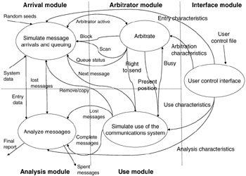
Figure 15.18: Basic structure of LAN simulator.

One of the critical modules of MALAN in terms of general characteristics modeling is the use module. Its major components are as follows:

1. ADD NEXT MESSAGE TO THE FILE. This process takes the next message from the processor that has the right to send and stores it in a file until it arrives at its destination.

2. SIMULATE TOPOLOGY. This routes the message through the simulation topology.

3. SIMULATE TRANSACTION DELAY. It simulates the passage of a message over a physical transmission line (link), including messages retransmitted.

4. SIMULATE MESSAGE ERRORS. This determines the number of retransmits and lost messages from information on the physical transmission line.

5. UNFILE MESSAGE. This process removes messages from the message file upon completion of message transmission.

6. SIMULATE STATUS CHANGE. This simulates the loss of a link or node.

Table 15.3 describes the composition of entities represented in this model. Each of the items in the table is an attribute of the model's entities. Attribute 1 is the event time; it contains the time at which the message will arrive. Attribute 2 is the event type, which distinguishes this event as an arrival, since there are other events that occur in the system. Attribute 3 is the source IU number or the designated IU that generated the message. Attribute 4 is the destination IU number and describes the ultimate destination of the message. Attribute 7 is the message size expressed in words. Attributes 17 and 18 are used when a message is too large to be sent in one packet. In this case, the message must be divided into a number of smaller messages, each with the same source, destination, and generation time. Attribute 17 is used to identify the sequence number of any multipacket message. Attribute 18 is used to identify the total number of packets in the entire message. With attributes 17 and 18, it can be determined when the complete message is received.

Table 15.3: Entries in the LAN Simulator Model

Attribute	Data Name	Data Type	Abbreviation
1	Event time	real	ETIM
2	Event type	real	ETYP
3	Source interface unit (IU) number	integer	SP
4	Destination interface unit (IU) number	integer	DP
5	Present interface unit (IU) number	integer	PP
6	Generation time	real	GT
7	Message size (words)	integer	MS
8	Message overhead length (bits)	integer	MO
9	Message wait time ∆t 1 (in processor queue)	real	WT1
10	Message wait time ∆t 2 (transit from queue to IU)	real	WT2
11	Message wait time ∆t 3 (within IU)	real	WT3
12	Message transfer time	real	TT
13	Message transfer time	real	XFER
14	Number of stops	integer	NS
15	Number of retransmits	integer	RT
16	Messages lost	integer	ML
17	Sequence number of multipacketed messages	integer	NMES
18	Number of parts to a packetized message	integer	PARTS
19	Message time to complete	integer	MTTC
20	Message priority	integer	MP
21	Message identification (ID) number	integer	MI

As with interarrival times, message size and message destination must be generated by the system. Here again, the data could be generated by measurements within the real system or by using theoretical distributions. Thus, part of the arrival module is devoted to drawing from distributions of message size and message destination and initializing the appropriate attributes. The only remaining function performed by this submode is to divide messages that exceed the maximum message size into a sequence of smaller messages. The total number of messages generated is placed in attribute 18 of each message. Each message receives a sequence number, attribute 17.

Once messages enter the system, they must be held in a waiting line or queue until the IU can transmit them. To facilitate this, a FIFO queue is formed to contain the waiting messages. In a real system, this queue would consume some real memory, which normally would be limited. In the simulated system, this limit must be taken into consideration. When queue memory is exceeded, appropriate action should be taken.

Appropriate action consists of: (1) waiting until sufficient memory is free to accommodate the message, (2) throwing away the message, and (3) overwriting an older message. Any of these can be selected in this submode.

Topology module description

The topology module consists mainly of a group of subroutines that facilitate the retrieval and modification of the data that physically describe the local computer network. These routines reside within the body of the simulation program with the exception of the initialization program, which is a separate entity.

15.3.9 Analysis module

The goal of the analysis module is to provide quantitative measures, which establish the effectiveness of distributed processing systems, and to provide statistical measures, which can be used to compare distributed processing systems having divergent design philosophies. To meet these goals, it is necessary to identify constant factors that unify distributed processing systems and derive statistical measures by which these factors can be compared. That is to say, a common language of analysis must be established by which a wide range of distributed systems can be described.

Establishing analysis criteria

In order to develop wide-ranging analysis criteria, it is necessary to identify those characteristics that are common among distributed processing systems. These common characteristics will be developed into statistical measures that analyze the relative merits of the underlying system. In developing common characteristics, three areas will be explored: (1) the basic physical structure of distributed processing networks, (2) the basic sequence of events, and (3) the overall function of distributed processing networks.

To provide flexibility and simplicity, most distributed processing systems have adopted a modular design philosophy. Modularity has resulted in a common physical structure, which allows the distributed processing systems to be divided into several functional components. These component parts can be examined and evaluated separately. Dividing the evaluation of a system into functional components allows more accurate analysis of the intermediate factors that contribute to the strengths and weaknesses of a system.

The basic functional components that form the physical structure of a typical distributed processing system are shown in Figure 15.19. This figure illustrates each distributed processing system in terms of the following components: (1) a number of processors that generate and consume messages, (2) a waiting line or queue containing messages that cannot be serviced immediately, (3) an interface unit that prepares messages for transmission, and (4) a communications network that performs the actual physical transmission of data. The physical implementation of these component parts differs widely from system to system. The outline presented in Figure 15.19 represents an accurate, generalized picture of distributed processing systems. The physical mapping presented in Figure 15.19 allows the identification of certain common features and checkpoints, which are discussed in subsequent paragraphs.

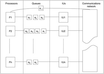
Figure 15.19: Functional components of a distributed processing system.

The primary structural feature of quantitative interest in Figure 15.19 is the queue, or waiting line. The length of these queues gives some quantitative information concerning the effectiveness of the underlying communications system. Exceptionally long or unbalanced queues could indicate the presence of system bottlenecks. Queues that grow and retreat wildly could suggest poor responsiveness to peak loads.

The basic components, which form the functional event structure in the typical distributed processing network, are shown in Figure 15.20. This figure reproduces the same general physical layout presented in Figure 15.19 but divides the passage of messages through the physical system into specific steps, or phases. The major events of interest along the message path of Figure 15.20 are: (1) a message arrives, (2) a message enters the queue, (3) a message leaves the queue, (4) a message becomes available to the interface unit, (5) a message starts transmission, (6) a message ends transmission, and (7) a message becomes available to the receiving processor.

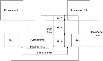
Figure 15.20: LAN evaluation metrics.

These common checkpoints are significant, because they allow time measurements that chart the passage of the message through the system. As long as a particular system accurately implements communication, timing becomes a most critical factor. That is, the speed at which accurately transmitted messages are completed is of primary interest. This series of checkpoints allows analysis of overall as well as intermediate delays imposed on the communications process.

The time between basic checkpoints and combinations of checkpoints gives rise to specific descriptive quantities, shown by the arrows in Figure 15.20. These quantities will be compiled for each simulation run on specific distributed processing networks. These are described in more detail, as follows:

1. System time is the time between message generation at the source processor and message reception by the sink processor. System time quantifies the total delay the distributed processing system imposes on a message.

2. Transfer time is the time that elapses between a message leaving the queue and its reception at the sink. Transfer time indicates the time required for the system to effect communications, disregarding the time spent waiting to commence the transfer process.

3. Transmit time is the time a message spends in the process of physical information transmission. This quantity indicates the actual timeliness of the low-level protocol and the speed of the physical transmission.

4. Wait time is the time that must be expended before a message begins transmission. This quantity is divided into four smaller quantities: wt1, wt2, wt3, and wt4, described as follows:

   • wt1 is the time a message spends in the queue.

   • wt2 is the interval between removing the message from the queue to the point at which the IU begins preparing the message for transmission.

   • wt3 accounts for the time required to prepare a message for transmission.

   • wt4 includes the time required to make the message available to the sink processor once the transmission is complete.

5. Overhead time equals the sum of wt2, wt3, and wt4. The overhead time is considered the time that must be yielded to the IU as the price of message transmission.

Analysis criteria can also be approached from a functional point of view. Functional criteria allow evaluation and comparison of the performance of distributed processing systems. These criteria fall into the following categories: (1) the amount of information carried by the communications system in unit time (i.e., throughput), (2) the amount of useful information transferred in unit time excluding overhead (i.e., information throughput), (3) the information lost in the communications process, (4) the amount of information overhead, and (5) the proportion of data that arrives late.

The throughput statistics quantify the total volume of information carried by a distributed processing system in unit time. This value is an overall indicator of the capacity and utilization of a distributed processing system. Unfortunately, the volume of real information transferred is reduced by the portion of overhead appended to the message. The overhead information is the part of a message that is attached by the distributed processing system to facilitate communication. The measurement of throughput that disregards overhead is called information throughput.

In addition to the overall flow of information through the system, we are interested in the loss of information. This loss can be the result of three conditions: (1) message loss because of a full queue, (2) message loss because of a bit(s) in error during transmission, and (3) message loss because of the casualty of a system component. These quantities will be computed as a percent of the total number of messages transmitted. A statistic relating total messages lost will also be computed.

Also of interest is the amount of overhead that is attached to each message. This quantity allows analysis of the degradation of system performance caused by overhead. This statistic expresses overhead as a percentage of the total information transferred.

A more sophisticated functional evaluation criterion is the data late statistics. This statistic evaluates the proportion of messages that arrives past the time of expiration. In a very practical sense, this measure is one that is of ultimate concern in real-time environments. If all messages arrive in their allotted time, the system is working within capacity and responds to the peak requirements demanded of it.

In summary, the criteria used for analysis are generated by three characteristics of distributed processing systems, as follows:

1. Basic physical structure. This characteristic yields criteria such as queue length, which results from the physical link between the processor and interface unit.

2. The event structure. This characteristic yields analysis criteria such as transmit time, which is the result of the requirement to physically transmit the data during some point in the communications cycle.

3. The overall function. This characteristic yields analysis criteria such as throughput, which results from the overall function of the system (i.e., to communicate).

Analysis criteria and simulation

From the point of view of statistical analysis, Figure 15.21 illustrates the essential nature of the model. The block on the left shows simulation messages arriving to the communications network from the real-time system. Messages in the simulation are not real system messages but are buffers of computer memory that contain information regarding the nature and history of the message. The central block shows simulation of messages passing through the communications network. During this passage, data, which capture the history of the message, are added to the simulated message. When the message is either complete (reaches its destination) or lost (failed to reach its destination), the message is analyzed by the analysis module shown as the block on the right.

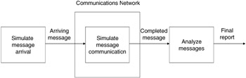
Figure 15.21: Simulated message flow graph.

During a simulation, many messages will take the path illustrated in Figure 15.22. A large number of messages are required in order to build up what is called statistical significance. This refers to the fact that a large sample of occurrences must be taken into consideration in order to eliminate any bias that may be produced by taking too small a random sample.

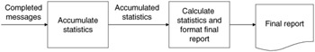
Figure 15.22: Analysis module functional diagram.

The structure of the software for collecting statistics and formatting the final report is also shown in Figure 15.22. During a simulation run, information from large numbers of completed messages will be accumulated and stored, and the memory occupied by these messages will be released. At the end of a simulation run, these accumulated data will be used in statistical calculations, which will be formatted and presented in the form of a final report.

Statistical output

The statistics generated by the system can be divided into three main groups: (1) time independent, (2) time persistent, and (3) periodic.

The time-independent statistics are from independent observations. The traditional mean and standard deviation can be calculated for this group. These data, which are accumulated during the simulation run, are as follows: (1) the sum of each observed piece of data, (2) the sum of each piece of data squared, (3) the number of observations, and (4) the maximum value observed. From the accumulated data, the mean, standard deviation, and maximum observed value will be calculated and formatted for the final report. These statistics will be provided for all the time-independent data points.

Time-persistent statistics are important when the time over which a parameter retains its value becomes critical. An example of this is a waiting line. If the line has ten members in it for 20 minutes and one member for 1 minute, the average is not (1 + 10)/2, or 5.5. This quantity would indicate that there were approximately five members present in the line for a 21-minute period. The true average is more like 20/21 × 10 + 1/20 × 1, or 9.57, or approximately 10. This is the time-persistent average. As can be seen in this case, the average is weighted by the time period over which the value persisted. There is a similar argument that can be made for the time-persistent standard deviation. These data, which are accumulated during a simulation for the time-persistent case, are as follows: (1) the sum of the observed value times the period over which it retained that value, (2) the sum of the observed value squared times the period over which it retained its value, (3) the maximum observed value, and (4) the total period of observation. From these accumulated data, the time-persistent mean, the time-persistent standard deviation, and the maximum observed value will be calculated and formatted for the final report. These statistics will be provided for all the time-persistent data points.

Periodic statistics are designed to yield a plot of observations as a function of time. This group of statistics affords a view of the system as it operates in time. Data are accumulated as in the previous two examples, except, rather than sums of statistics, an individual data point graph of time versus the value of the data points will be plotted. These plots will be produced for all groups of periodic statistics. Some example plots for evaluations performed on the HXDP and token ring networks are shown in Figure 15.23.

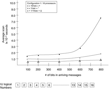
Figure 15.23: Example performance evaluation plots.

---