| A pivot table is the most powerful means of analyzing data available in Excel. That might sound over the top, but it's true. Consider that a pivot table enables you to View a data field (such as age, weight, revenues, costs, and so on) as a sum, an average, a standard deviation, a count of cases, and seven other types of summary Categorize the records according to many different fields (such as sex, product line, political affiliation, region, and so on) Combine and recombine categories (such as male Republicans, or routers sold from northwest offices) just by dragging a cell Base the pivot table on a list in an Excel workbook, or an external data source such as a database or a data cube Display the data in a chart in addition to a table--a chart that pivots its dimensions just as a pivot table does
It starts to become apparent that you've put your hands on a powerful tool indeed. But if you've used pivot tables much, you know that they can give you more information than you need. Suppose that your pivot table analyzes revenues and costs by region and product. An example appears in Figure 2.16. Figure 2.16. Pivot tables don't always offer the perfect format for reports. 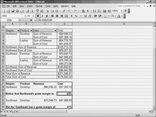
If you wanted to insert comments among the results of the pivot table, you'd be out of luck. Instead, you have to copy the results you want into other cells and insert your comments where you want them. In Figure 2.16, in cells A27:D34, the user wants to focus on costs and revenues for Desktops in both regions and intersperse comments about the gross margin. The GETPIVOTDATA function is ideal for this. The function returns a value from a pivot table to the cell where you enter it. Its syntax depends on the Excel version you're using. Using GETPIVOTDATA in Excel 97 and Excel 2000 The syntax is GETPIVOTDATA(pivot table, name)
Here, the pivot table argument is a reference to a pivot table. It can be any of these: A cell that the pivot table occupies, such as $B$14 A range name that identifies the full pivot table, such as PivotRange, where the name itself might refer to $A$11:$D$25, as in Figure 2.16 The name of a pivot table such as PivotTable3, as specified in the pivot table's options
The name argument is one or more items in the pivot table, entered as a single string. Using the data as shown in Figure 2.16, you could enter =GETPIVOTDATA($A$11,"Northwest Desktop Sum of Cost")
to get the value shown in cell D13. Notice that the name argument includes items from two different fields (the Northwest item from the Region field, and the Desktop item from the Product field), as well as the name of the data field (Sum of Cost). When a pivot table has more than one data field, you have to specify the one you want--otherwise, you'll get a #REF! error. Using GETPIVOTDATA in Excel 2002 and Excel 2003 The syntax is GETPIVOTDATA(data field, pivot table, field1, item1, field2, item2 . . .)
You can specify as many as 14 fields and associated items in the argument list. Just as in the Excel 97 and 2000 version, you specify the pivot table you're after with the pivot table argument: a cell in the pivot table, or the name of the range the pivot table occupies, or the name of the pivot table. In contrast to the Excel 97 and 2000 versions, the arguments in Excel 2002 and 2003 call out the fields separately, instead of all together in a single name argument. One possible 2002/2003 version of the formula to return the value in cell D13 of Figure 2.16 is =GETPIVOTDATA("Sum of Cost", $A$11, "Region","Northwest","Product","Desktop")
Entering GETPIVOTDATA Automatically Excel 2002 and 2003 give you a way to avoid the tedium of entering the arguments for GETPIVOTDATA. Just enter an equal sign in a cell and then click in a data field cell in a pivot table. Again using the layout in Figure 2.16, you might select cell D37, type an equal sign, and then click any cell in the range D12:D25. Excel generates the GETPIVOTDATA arguments automatically. For example, if you typed an equal sign in some blank cell and then clicked in cell D18, Excel would generate this formula for you: =GETPIVOTDATA("Sum of Revenue",$A$11,"Region","Southeast","Product","Desktop")
This automatic formula generation is optional (although it is the default option). If you want a simple cell link instead--such as =D18--you can just type the cell reference instead of using point and click. Or toggle the option by taking these steps: - If necessary, choose View, Toolbars and show the PivotTable toolbar. (This step is needed only if you want to use the PivotTable toolbar and it's not currently visible.)
- Choose Options, Customize and click the Commands tab.
- Click Data in the Categories list box.
- In the Commands list box, scroll down until you see Generate GetPivotData.
- Click on Generate GetPivotData, hold down the mouse button, and drag it to a toolbar. Release the mouse button.
Now you can click the Generate GetPivotData button to toggle the option on and off. Pivoting the Table: Why Use GETPIVOTDATA? It might seem pointless to use GETPIVOTDATA, with all its arguments, instead of a simple cell link. Figure 2.17 shows a pivot table along with two formulas. Both formulas return the same value from the pivot table. Figure 2.17. Using GETPIVOTDATA looks a lot more tedious than a simple cell link. 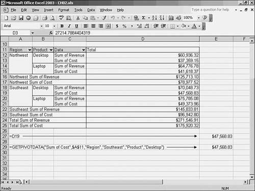
The formula in E27 is =D19. It is a simple cell link, and displays whatever value is in D19. In Figure 2.17, that value is $47,568.83. The formula in E29 is =GETPIVOTDATA("Sum of Cost",$A$11,"Region","Southeast","Product","Desktop")
This lengthy formula also returns the value in D19, $47,568.83, but it does so by way of naming the fields and items. Figure 2.18 shows what happens when you decide to pivot the table, making Product a column field instead of an inner row field as in Figure 2.17. After pivoting the table, as Figure 2.18 shows, the simple cell link in E27 still points to cell D19, but because it's empty, the link returns $0.00. However, the GETPIVOTDATA function still looks up its value using field and item names, so it continues to return the value it did before pivoting. Figure 2.18. The pivot table no longer occupies cell D19, and the simple cell link now returns zero. 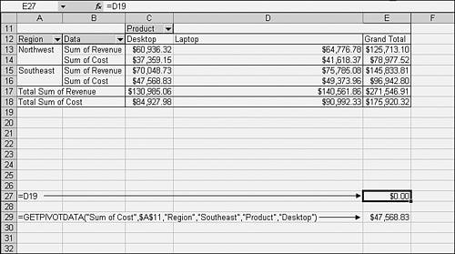
GETPIVOTDATA is no cure-all. If you rename a field (for example, rename Product to Product Line) or an item (for example, rename Desktop to Desktops), GETPIVOTDATA won't know where to look to find the data field value you're after. |