Section 10.2. Data Warehousing
10.2. Data WarehousingThe purpose of this book is not to devote half a chapter to covering the complex issues linked to data warehousing . Many books on the topic of data warehousing have been written, some of them generic (Ralph Kimball's The Data Warehouse Toolkit and Bill Inmon's Building the Data Warehouse , both published by John Wiley & Sons, are probably the two best-known titles), some of them specific to a DBMS engine. There has been something of a religious war between the followers of Inmon, who advocates a clean 3NF design of enormous data repositories used by decision-support systems, and the supporters of Kimball, who believes that data warehouses are a different world with different needs, and that therefore the 3NF model, in spite of its qualities in the operational world, is better replaced with dimensional modeling , in which reference data is happily denormalized. As most of this book advocates and assumes a clean 3NF design, I will deal hereafter more specifically with dimensional models, to study their strengths and the reason for their popularity, but also their weaknesses. I will, in particular, examine the interactions between operational data stores ("production databases " to the less enlightened) and decision-support systems, since data doesn't fall from heaven, unless you are working for NASA or a satellite operating company, and what you load into dimensional models has to come from somewhere. Understand that it is not because one is using the SQL language against "tables" that one is operating in the relational world. 10.2.1. Facts and Dimensions: the Star SchemaThe principle of dimensional modeling is to store measurement values, whether they are quantities, amounts, or whatever you can imagine into big fact tables . Reference data is stored into dimension tables that mostly contain self-explanatory labels and that are heavily denormalized. There are typically 5 to 15 dimensions, each with a system-generated primary key, and the fact table contains all the foreign keys. Typically, the date associated with a series of measures (a row) in the fact table will not be stored as a date column in the fact table, but as a system-generated number that will reference a row in the date_dimension table in which the date will be declined under all possible forms. If we take, for instance, the traditional starting date of the Unix world, January 1, 1970, it would typically be stored in date_dimension as:
Every row that refers to something having occurred on January 1, 1970 in the fact table would simply store the 12345 key. The rationale behind such an obviously non-normalized way of storing data is that, although normalization is highly important in environments where data is changed, because it is the only way to ensure data integrity, the overhead of storing redundant information in a data warehouse is relatively negligible since dimension tables contain very few rows compared to the normalized fact table. For instance, a one-century date dimension would only hold 36,525 rows. Moreover, argues Dr. Kimball, having only a fact table surrounded by dimension tables as in Figure 10-3 (hence the "star schema " name) makes querying that data extremely simple. Queries against the data tend to require very few joins, and therefore are very fast to execute. Figure 10-3. A simple star schema, showing primary keys (PK) and foreign keys (FK) Anybody with a little knowledge of SQL will probably be startled by the implication that the fewer the joins, the faster a query runs. Jumping to the defense of joins is not, of course, to recommend joining indiscriminately dozens of tables, but unless you have had a traumatic early childhood experience with nested loops on big, unindexed tables, it is hard to assert seriously that joins are the reason queries are slow. The slowness comes from the way queries are written; in this light, dimensional modeling can make a lot of sense, and you'll see why as you progress through this chapter. The design constraints of dimensional modeling are deliberately read-oriented, and consequently they frequently ignore the precepts of relational design. 10.2.2. Query ToolsThe problem with decision-support systems is that their primary users have not the slightest idea how to write an SQL query, not even a terrible one. They therefore have to use query tools for that purpose, query tools that present them with a friendly interface and build queries for them. You saw in Chapter 8 that dynamically generating an efficient query from a fixed set of criteria is a difficult task, requiring careful thought and even more careful coding. It is easy to understand that when the query can actually be anything, a tool can only generate a decent query when complexity is low. The following piece of code is one that I saw actually generated by a query tool (it shows some of the columns returned by a subquery in a from clause): ... FROM (SELECT ((((((((((((t2."FOREIGN_CURRENCY" || CASE WHEN 'tfp' = 'div' THEN t2."CODDIV" WHEN 'tfp' = 'ac' THEN t2."CODACT" WHEN 'tfp' = 'gsd' THEN t2."GSD_MNE" WHEN 'tfp' = 'tfp' THEN t2."TFP_MNE" ELSE NULL END ) || CASE WHEN 'Y' = 'Y' THEN TO_CHAR ( TRUNC ( t2."ACC_PCI" ) ) ELSE NULL END ) || CASE WHEN 'N' = 'Y' THEN t2."ACC_E2K" ELSE NULL END ) || CASE WHEN 'N' = 'Y' THEN t2."ACC_EXT" ELSE NULL END ) || CASE ... It seems obvious from this sample's select list that at least some "business intelligence" tools invest so much intelligence on the business side that they have nothing left for generating SQL queries. And when the where clause ceases to be trivialforget about it! Declaring that it is better to avoid joins for performance reasons is quite sensible in this context. Actually, the nearer you are to the "text search in a file" (a.k.a. grep) model, the better. And one understands why having a "date dimension" makes sense, because having a date column in the fact table and expecting that the query tool will transform references to "Q1" into "between January 1 and March 31" to perform an index range scan requires the kind of faith you usually lose when you stop believing in the Tooth Fairy. By explicitly laying out all format variations that end users are likely to use, and by indexing all of them, risks are limited. Denormalized dimensions, simple joins, and all-round indexing increase the odds that most queries will execute in a tolerable amount of time, which is usually the case. Weakly designed queries may perform acceptably against dimensional models because the design complexity is much lower than in a typical transactional model. 10.2.3. Extraction, Transformation, and LoadingIn order for business users to be able to proactively leverage strategic cost-generating opportunities (if data warehousing literature is to be believed), it falls on some poor souls to ensure the mundane task of feeding the decision-support system. And even if tools are available, this feeding is rarely an easy task. 10.2.3.1. Data extractionData extraction is not usually handled through SQL queries. In the general case, purpose-built tools are used: either utilities or special features provided by the DBMS, or dedicated third-party products. In the unlikely event that you would want to run your own SQL queries to extract information to load into a data warehouse, you typically fall into the case of having large volumes of information, where full table scans are the safest tactic. You must do your best in such a case to operate on arrays (if your DBMS supports an array interfacethat is fetching into arrays or passing multiple values as a single array), so as to limit round-trips between the DBMS kernel and the downloading program. 10.2.3.2. TransformationDepending on your SQL skills, the source of the data, the impact on production systems, and the degree of transformation required, you can use the SQL language to perform a complex select that will return ready-to-load data, use SQL to modify the data in a staging area, or use SQL to perform the transformation at the same time as the data is uploaded into the data warehouse. Transformations often include aggregates, because the granularity required by decision support systems is usually coarser than the level of detail provided by production databases. Typically, values may be aggregated by day. If transformation is not more complicated than aggregation, there is no reason for performing it as a separate operation. Writing to the database is much costlier than reading from it, and updating the staging area before updating the data warehouse proper may be adding an unwanted costly step. Such an extra step may be unavoidable, though, when data has to be compounded from several distinct operational systems; I can list several possible reasons for having to get data from different unrelated sources:
The assemblage of data from several sources should be done, as much as possible, in a single step, using a combination of set operators such as union and of in-line viewssubqueries in the from clause. Multiple passes carry a number of risks and should not be directly applied to the target data warehouse. The several-step update of tables, with null columns being suddenly assigned values is an excellent recipe for wreaking havoc at the physical level. When data is stored in variable length, as is often the case with character information and sometimes with numeric information as well (Oracle is an example of such a storage strategy), it will invariably lead to some of the data being relegated to overflow pages, thus compromising the efficiency of both full scans and indexed accesses, since indexes usually point to the head part of a row. Any pointer to an overflow area will mean visiting more pages than would otherwise be necessary to answer a given question, and will be costly. If the prepared data is very simply inserted into the target data warehouse tables, data will be properly reorganized in the process. It is also quite common to see several updates applied to different columns of the same table in turn. Whenever possible, perhaps with help from the case construct, always update as many columns in one statement as possible. Multiple massive updates applied to a table often wreak havoc at the physical level. 10.2.3.3. LoadingIf you build your data warehouse (or data mart, as others prefer to say) according to the rules of dimensional modeling, all dimensions will use artificial, system-generated keys for the purpose of keeping a logical track over time of items that may be technically different but logically identical. For instance, if you manufacture consumer electronics, a new model with a new reference may have been designed to replace an older model, now discontinued. By using the same artificial key for both, you can consider them as a single logical entity for analysis. The snag is that the primary keys in your operational database will usually have different values from the dimension identifiers used in the decision support system, which becomes an issue not with dimension tables but with fact tables. You have no reason to use surrogate keys for dates in your operational system. In the same way, the operational system doesn't necessarily need to record which electronic device model is the successor to another. Dimension tables are, for the most part, loaded once and rarely updated. Dimensional modeling rests partly on the assumption that the fast-changing values are the ones stored in fact tables. As a result, for every row you need to insert into the fact table, you must retrieve (from the operational database primary key) the value of the corresponding surrogate, system-generated key for each of the dimensionswhich necessarily means as many joins as there are different dimensions. Queries against the decision support system may require fewer joins, but loading into the decision support system will require many more joins because of the mapping between operational and dimensional keys. The advantage of simpler queries against dimensional models is paid for by the disadvantage of complex preparation and loading of the data. 10.2.3.4. Integrity constraints and indexesWhen a DBMS implements referential integrity checking, it is sensible to disable that checking during data load operations. If the DBMS engine needs to check for each row that the foreign keys exist, the engine does double the amount of work, because any statement that uploads the fact table has to look for the parent surrogate key anyway. You might also significantly speed up loading by dropping most indexes and rebuilding them after the load, unless the rows loaded represent a small percentage of the size of the table that you are loading, as rebuilding indexes on very large tables can be prohibitively expensive in terms of resources and time. It would however be a potentially lethal mistake to disable all constraints, and particularly primary keys. Even if the data being loaded has been cleaned and is above all reproach, it is very easy to make a mistake and load the same data twicemuch easier than trying to remove duplicates afterwards. The massive upload of decision-support systems is one of the rare cases when temporarily altering a schema may be tolerated. 10.2.4. Querying Dimensions and Facts: Ad Hoc ReportsIf query tools are seriously helped by removing anything that can get in their way, such as evil joins and sophisticated subqueries, there usually comes a day when business users require answers that a simplistic schema cannot provide. The dimensional model is then therefore duly "embellished" with mini-dimensions , outriggers , bridge tables , and all kinds of bells and whistles until it begins to resemble a clean 3NF schema, at which point query tools are beginning to suffer. One day, a high-ranking user tries something daringand the next day the problem is on the desk of a developer, while the tool-generated query is still running. Time for ad hoc queries and shock SQL! It is when you have to write ad hoc queries that it is time to get back to dimensional modeling and see the SQL implications . Basically, dimensions represent the breaks in a report. If an end user often wants to see sales by product, by store, and by month, then we have three dimensions involved: the date dimension that has been previously introduced, the product dimension, and the store dimension. Product and store can be denormalized to include information such as product line, brand, and category in one case, and region, surface, or whatever criterion is deemed to be relevant in the other case. Sales amounts are, obviously, facts. A key characteristic of the star schema is that we are supposed to attack the fact table through the dimensions such as in Figure 10-4; in the previous example, we might for instance want to see sales by product, store, and month for dairy products in the stores located in the Southwest and for the third quarter. Contrarily to the generally recommended practice in normalized operational databases, dimension tables are not only denormalized, but are also strongly indexed. Indexing all columns means that, whatever the degree of detail required (the various columns in a location dimension, such as city, state, region, country, area, can be seen as various levels of detail, and the same is true of a date dimension), an end user who is executing a query will hit an index. Remember that dimensions are reference tables that are rarely if ever updated, and therefore there is no frightful maintenance cost associated with heavy indexing. If all of your criteria refer to data stored in dimension tables, and if they are indexed so as to make any type of search fast, you should logically hit dimension tables first and then locate the relevant values in the fact table. Figure 10-4. The usual way of querying tables in the dimensional model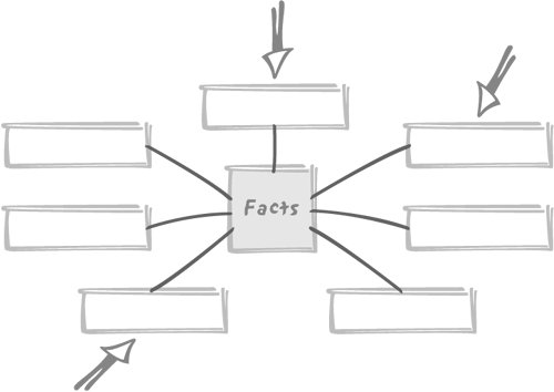 Hitting dimensions first has very strong SQL implications that we must well understand. Normally, one accesses particular rows in a table through search criteria, finds some foreign keys in those rows, and uses those foreign keys to pull information from the tables those keys reference. To take a simple example, if we want to find the phone number of the assistant in the department where Owens works, we shall query the table of employees basing our search on the "Owens" name, find the department number, and use the primary key on the table of departments to find the phone number. This is a classic, nested-loop join case. With dimensional modeling, the picture totally changes. Instead of going from the referencing table (the employees) to the referenced table (the departments), naturally following foreign keys, we start from the reference tablesthe dimensions. To go where? There is no foreign key linking a dimension to the fact table: the opposite is true. It is like looking for the names of all the employees in a department when all you know is the phone number of the assistant. When joining the fact table to the dimension, the DBMS engine will have to go through a mechanism other than the usual nested loopperhaps something such as a hash join. Another peculiarity of queries on dimensional models is that they often are perfect examples of the association of criteria that's not too specific, with a relatively narrow intersection to obtain a result set that is not, usually, enormous. The optimizer can use a couple of tactics for handling such queries. For instance:
In such a case, visiting the fact table at an early stage, which also means after a first dimension, may be a mistake. Some products such as Oracle implement an interesting algorithm, known in Oracle's case as the "star transformation." We are going to look next at this transformation in some detail, including characteristics that are peculiar to Oracle, before discussing how such an algorithm may be emulated in non-Oracle environments. Dimensional modeling is built on the premise that dimensions are the entry points. Facts must be accessed last. 10.2.4.1. The star transformationThe principle behind the star transformation is, as a very first step, to separately join the fact table to each of the dimensions for which we have a filtering condition. The transformation makes it appear that we are joining several times to the fact table, but appearances are deceiving. What we really want is to get the addresses of rows from the fact table that match the condition on each dimension. Such an address, also known as a rowid (accessible as a pseudo-column with Oracle; Postgres has a functionally equivalent oid) is stored in indexes. All we need to join, therefore, are three objects:
Even though the fact table appears several times in a star query, we will not hit the same data or index pages repeatedly. All the separate joins will involve different indexes, and all storing rowids referring to the same tablebut otherwise those indexes are perfectly distinct objects. As soon as we have the result of two joins, we can combine the two resulting sets of rowids, discarding everything that doesn't belong to the intersection of the two sets for an and condition or retaining everything for an or condition. This step is further simplified if we are using bitmap indexes , for which simple bit-wise operations are all that is required to select our final set of rowids that refer to rows satisfying our conditions. Once we have our final, relatively small set of resulting rowids, then we can fetch the corresponding rows from the fact table that we are actually visiting for the very first time. Bitmap indexes, as their name says, index values by keeping bitmaps telling which rows contain a particular value and which do not. Bitmap indexes are particularly appropriate to index low-cardinality columns; in other words, columns in which there are few distinct values, even if the distribution of those values is not particularly skewed. Bitmap indexes were not mentioned in previous chapters for an excellent reason: they are totally inappropriate for general database operations. There is a major reason for avoiding them in a database that incurs normal update activity: when you update a bitmap, you have to lock it. Since this type of index is designed for columns with few distinct values, you end up preventing changes to many, many rows, and you get a behavior that lies somewhere between page locking and table locking, but much closer to table locking. For read-only databases, however, bitmap indexes may prove useful. Bitmap indexes are quickly built during bulk loads and take much less storage than regular indexes. 10.2.4.2. Emulating the star transformationAlthough automated star transformation is a feature that enables even poorly generated queries to perform efficiently, it is quite possible to write a query in a way that will induce the DBMS kernel to execute it in a similar, if not exactly identical, fashion. I must plead guilty to writing SQL statements that are geared at one particular result. From a relational point of view, I would deserve to be hanged high. On the other hand, dimensional modeling has nothing to do with the relational theory. I am therefore using SQL in a shamelessly unrelational way. Let's suppose that we have a number of dimension tables named dim1, dim2, ...dimn. These dimension tables surround our fact table that we shall imaginatively call facts. Each row in facts is composed of key1, key2, ...keyn, foreign keys respectively pointing to one dimension table, plus a number of values (the facts) val1, val2, ...valp. The primary key of facts is defined as a composite key, and is simply made of key1 to keyn. Let's further imagine that we need to execute a query that satisfies conditions on some columns from dim1, dim2, and dim3 (they may, for instance, represent a class of products, a store location, and a time period). For simplicity, say that we have a series of and conditions, involving col1 in dim1, col2 in dim2 and col3 in dim3. We shall ignore any transformation, aggregate or whatever, and limit our creative exercise to returning the appropriate set of rows in as effective a way as possible. The star transformation mostly aims to obtain in an efficient way the identifiers of the rows from the fact table that will belong to our result set, which may be the final result set or an intermediate result set vowed to further ordeals. If we start with joining dim2 to facts, for instance: select ... from dim2, facts where dim2.key2 = facts.key2 and dim2.col2 = some value then we have a major issue if we have no Oracle rowid, because the identifiers of the appropriate rows from facts are precisely what we want to see returned. Must we return the primary key from facts to properly identify the rows? If we do, we hit not only the index on facts(key2), but also table facts itself, which defeats our initial purpose. Remember that the frequently used technique to avoid an additional visit to the table is to store the information we need in the index by adding to the index the columns we want to return. So, must we turn our index on facts(key2) into an index on facts(key2, key3...keyn)? If we do that, then we must apply the same recipe to all foreign keys! We will end up with n indexes that will each be of a size in the same order of magnitude as the facts table itself, something that is not acceptable and that forces us to read large amounts of data while scanning those indexes, thus jeopardizing performance. What we need for our facts table is a relatively small row identifiera surrogate key that we may call fact_id. Although our facts table has a perfectly good primary key, and although it is not referenced by any other table, we still need a compact technical identifiernot to use in other tables, but to use in indexes. With our system-generated fact_id column, we can have indexes on (key1, fact_id), (key2, fact_id)...(keyn, fact_id) instead of on the foreign keys alone. We can now fully write our previous query as: select facts.fact_id from dim2, facts where dim2.key2 = facts.key2 and dim2.col2 = some value This version of the query no longer needs the DBMS engine to visit anything but the index on col2, the dimension table dim2, and the facts index on (key2, fact_id). Note that by applying the same trick to dim2 (and of course the other dimension tables), systematically appending the key to indexes on every column, the query can be executed by only visiting indexes. Repeating the query for dim1 and dim3 provides us with identifiers of facts that satisfy the conditions associated with these dimensions. The final set of identifiers satisfying all conditions can easily be obtained by joining all the queries: select facts1.fact_id from (select facts.fact_id from dim1, facts where dim1.key1 = facts.key1 and dim1.col1 = some value ) facts1, (select facts.fact_id from dim2, facts where dim2.key2 = facts.key2 and dim2.col2 = some other value ) facts2, (select facts.fact_id from dim3, facts where dim3.key3 = facts.key3 and dim3.col3 = still another value ) facts3 where facts1.fact_id = facts2.fact_id and facts2.fact_id = facts3.fact_id Afterwards, we only have to collect from facts the rows, the identifiers of which are returned by the previous query. The technique just described is, of course, not specific to decision-support systems. But I must point out that we have assumed some very heavy indexing, a standard fixture of data marts and, generally speaking, read-only databases. In such a context, putting more information into indexes and adding a surrogate key column can be considered as "no impact" changes. You should be most reluctant in normal (including in the relational sense!) circumstances to modify a schema so significantly to accommodate queries. But if most of the required elements are already in place, as in a data warehousing environment, you can certainly take advantage of them. 10.2.4.3. Querying a star schema the way it is not intended to be queriedAs you have seen, the dimensional model is designed to be queried through dimensions. But what happens when, as in Figure 10-5, our input criteria refer to some facts (for instance, that the sales amount is greater than a given value) as well as to dimensions? Figure 10-5. A maverick usage of the dimension model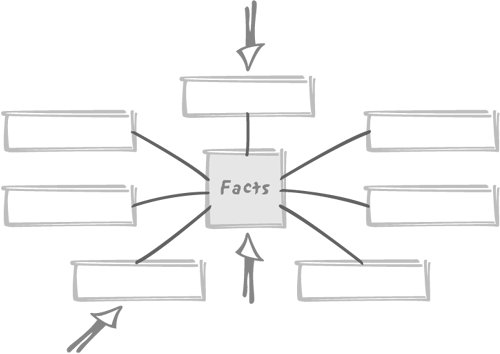 We can compare such a case to the use of a group by. If the condition on the fact table applies to an aggregate (typically a sum or average), we are in the same situation as with a having clause: we cannot provide a result before processing all the data, and the condition on the fact table is nothing more than an additional step over what we might call regular dimensional model processing. The situation looks different, but it isn't. If, on the contrary, the condition applies to individual rows from the fact table, we should consider whether it would be more efficient to discard unwanted facts rows earlier in the process, in the same way that it is advisable to filter out unwanted rows in the where clause of a query, before the group by, rather than in the having clause that is evaluated after the group by. In such a case, we should carefully study how to proceed. Unless the fact column that is subjected to a condition is indexeda condition that is both unlikely and unadvisableour entry point will still be through one of the dimensions. The choice of the proper dimension to use depends on several factors; selectivity is one of them, but not necessarily the most important one. Remember the clustering factor of indexes, and how much an index that corresponds to the actual, physical order of rows in the table outperforms other indexes (whether the correspondence is just a happy accident of the data input process, or whether the index has been defined as constraining the storage of rows in the table). The same phenomenon happens between the fact table and the dimensions. The order of fact rows may happen to match a particular date, simply because new fact rows are appended on a daily basis, and therefore those rows have a strong affinity to the date dimension. Or the order of rows may be strongly correlated to the "location dimension" because data is provided by numerous sites and processed and loaded on a site-by-site basis. The star schema may look symmetrical, just as the relational model knows nothing of order. But implementation hazards and operational processes often result in a break-up of the star schema's theoretical symmetry. It's important to be able to take advantage of this hidden dissymmetry whenever possible. If there is a particular affinity between one of the dimensions to which a search filter must be applied and to the fact table, the best way to proceed is probably to join that dimension to the fact table, especially if the criterion that is applied to the fact table is reasonably selective. Note that in this particular case we must join to the actual fact table, obviously through the foreign key index, but not limit our access to the index. This will allow us to directly get a superset of our target collection of rows from the fact table at a minimum cost in terms of visited pages, and check the condition that directly applies to fact rows early. The other criteria will come later. The way data is loaded to a star schema can favor one dimension over all others. 10.2.5. A (Strong) Word of CautionDimensional modeling is a technique, not a theory, and it is popular because it is well-suited to the less-than-perfect (from an SQL[*] perspective) tools that are commonly used in decision support systems, and because the carpet-indexing (as in "carpet-bombing") it requires is tolerable in a read-only systemread-only after the loading phase, that is. The problem is that when you have 10 to 15 dimensions, then you have 10 to 15 foreign keys in your fact table, and you must index all those keys if you want queries to perform tolerably well. You have seen that dimensions are mostly static and not enormous, so indexing all columns in all dimensions is no real issue. But indexing all columns may be much more worrisome with a fact table, which can grow very big: just imagine a large chain of grocery stores recording one fact each time they sell one article. New rows have to be inserted into the fact table very regularly. You saw in Chapter 3 that indexes are extremely costly when inserting; 15 indexes, then, will very significantly slow down loading. A common technique to load faster is to drop indexes and then recreate them (if possible in parallel) once the data is loaded. That technique may work for a while, but re-indexing will inexorably take more time as the base table grows. Indexing requires sorting, and (as you might remember from the beginning of this chapter) sorts belong to the category of operations that significantly suffer when the number of rows increases. Sooner or later, you will discover that the re-creation of indexes takes way too much time, and you may well also be told that you have users who live far, far away who would like to access the data warehouse in the middle of the night.
Users that want the database to be accessible during a part of the night mean a smaller maintenance window for loading the decision support system. Meanwhile, because recreating indexes takes longer as data accumulates into the decision support database, loading times have a tendency to increase. Instead of loading once every night, wouldn't it be possible to have a continuous flow of data from operational systems to the data warehouse? But then, denormalization can become an issue, because the closer we get to a continuous flow, the closer we are to a transactional model, with all the integrity issues that only proper normalization can protect against. Compromising on normalization is acceptable in a carefully controlled environment, an ivory tower. When the headquarters are too close to the battlefield, they are submitted to the same rules. |
EAN: 2147483647
Pages: 143