Calc Basics

---

The toolbars in Open Office Calc are in a particular order with each toolbar containing specific tools for specific functions. The toolbars are listed here:

• A Menu toolbar

• A Function toolbar

• An Object toolbar

• A Calculation toolbar

The Menu toolbar contains Calc’s main menus. The Menu toolbar provides user access to basic functions such as Open, Save, Copy, Cut, Paste, and so on. These functions are common to all Open Office applications. In fact, with almost any application, you will see the same or very similar items grouped under the File menu. The Object toolbar consists of a set of tools that are specific to calculation and cell formatting (number format, text alignment, borders). These are the buttons that are unique to Calc and will not be found in other Open Office applications. Finally, the Calculation toolbar enables a user to enter his own specific formulas for calculations. This toolbar also displays the current cursor position within the spreadsheet .

These toolbars can be customized. One way to do this is to right-click on any of the toolbars and select Visible Buttons, as shown in Figure 9.3. This enables you to choose what buttons are shown in the toolbar and which buttons are not shown.

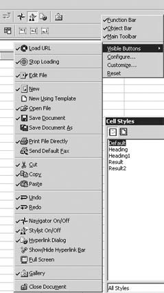
Figure 9.3: Choosing Visible Buttons.

When you right-click on any toolbar, all the toolbars are displayed in a list. The visible toolbars have a checkmark by their names on the list. You can choose to display or not display an entire toolbar by checking or unchecking it in the list. You can also right-click on any toolbar and select Configure. This will enable you access to all of the configuration options in one convenient screen.

On the left of the screen you will see the toolbar, shown in Figure 9.4. This toolbar provides a number of specialized tools for use with a spreadsheet. We will explore these functions in more depth later in this chapter.

Figure 9.4: The toolbar.

The spreadsheet is represented as a grid composed of rows and columns creating cells. A cell is referenced by its column (vertical reference), given as a letter such as A, B…Z, and its line (horizontal reference) is given as a number such as 1, 2…300. A particular cell might be identified as B10. This is the same as identifying a specific cell within Microsoft Excel. An individual cell contains some sort of data. You will usually place a number in a cell, as numeric data is usually used in a spreadsheet. However, you also can enter text directly into any cell. This is useful for labeling data.

Basic Calculations

Performing calculations is the reason for a spreadsheet program. Therefore, we should probably delve right into entering data and performing calculations. First we are going to create a simple spreadsheet for a small business. We will organize our spreadsheet in rows that designate types of expenses and columns that indicate months, as shown in Figure 9.5. Remember that you need to click inside a cell and then you can enter text or numbers. You should also note that if you enter January in the first month cell and then click on the lower-right corner of that cell and drag across, the subsequent cells will be filled automatically with the appropriate month, as you also see in Figure 9.5. This particular feature of Calc behaves in exactly the same manner as Excel. You can do the same thing with numeric values in a cell and drag your mouse. The values will be incremented by 1 in each cell. This works very much the same in Excel, but the actual values will be duplicated to subsequent cells rather than a steady increment of the value. In both Excel and Calc this function is called AutoFill, since it automatically fills in appropriate data.

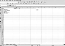
Figure 9.5: A simple spreadsheet.

Now enter some figures for the various cells. For our purposes, the actual numbers you enter are irrelevant, but of course those numbers would be very important in a real-world business situation. You can make your column headers a different font, perhaps bold. This will help them stand out from your actual data. You can accomplish this by highlighting an individual cell or an entire row and then selecting the formatting options you want to implement. This is how formatting cells is done in Excel, so you should have no problem with this task. Once you are done, your spreadsheet should look very much like the one in Figure 9.6.

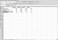
Figure 9.6: Sample data in your spreadsheet.

Now we have our data in a very neat looking spreadsheet, but that is only the beginning of what anyone wants from spreadsheets. Simply typing in the data is not particularly exciting. We want to manipulate the data and produce statistics, answers, and such. In short, we want to do some number crunching. Now we will begin to manipulate the data in a variety of ways. The simplest calculation we can do is to total the values in a given row or column. If you click once in the first blank cell after a row or column of numbers, you can then go to the toolbar and click on the summation symbol, shown in Figure 9.7. Notice that we mentioned rows or columns. You can total up either a row or a column. In fact, all of the functions available in either Calc or Excel can be executed against data from either a row or a column.

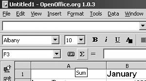
Figure 9.7: The summation button.

You will then be shown a formula in the formula bar, and you can choose to either accept it or reject it, as shown in Figure 9.8. If you choose to accept it, the answer to that formula will be displayed in the cell you initially clicked on.

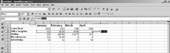
Figure 9.8: The summation formula.

This is very similar to how summation works in Excel. The buttons even look the same in both applications. The difference is that in Excel you don’t have the option to accept or reject the choice you make. Once you click the summation button, the formula is inserted, and the calculation is done.

This, however, is a rather simple calculation. You will probably require more advanced calculations. Before we move on to other calculations, we want to make sure we will remember what this column we just generated represents. Numbers without labels quickly become meaningless. For that reason, you probably want to label the column you put the sum in. You might give it some label such as Total. Once you have done that, you might notice the button to the left of the summation button. It is referred to as the Autopilot button. When you press it you will be shown a list of built-in functions you can insert into your spreadsheet, as shown in Figure 9.9.

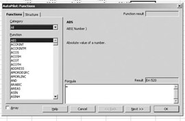
Figure 9.9: Functions.

There are literally dozens of calculations/functions listed here. Many, if not most, of the calculations you will require are listed here. For our purposes, scroll down the list until you find a function named STDEV. This is the standard deviation. If you are not familiar with basic statistics, don’t worry. Calc will do all the number crunching for you. Conceptually, standard deviation is simply an average of how much each individual item in a sample deviates from the sample’s average. This tells us whether or not the mean is a useful statistic. A high standard deviation means that there really was no norm for that data group.

When you have selected the STDEV function, press the next button and you will see a screen like the one in Figure 9.10, where you can enter the various cells you want to compute standard deviation for.

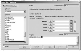
Figure 9.10: Performing calculations.

You should notice that on the right side, in the lower third of the screen, the result for the numbers you picked is already being displayed. When you click OK, this result will be put into the spreadsheet. If you should later change the value of any of the cells that you included in the standard deviation calculation, the calculation’s total will automatically be revised to match the changed or new data. Also note that you can also get to these functions from the drop-down menu by selecting Insert and Functions. This is the way you get to similar functions in Microsoft Excel. In addition to average and standard deviation, you can see that there are dozens of other built-in functions you can use.

There is a large number of functions you can choose in Calc, some of which might be beyond some readers’ mathematical understanding. However, Table 9.1 lists many of the commonly used functions and what they do.

Table 9.1: Calc Functions

Function	Purpose
AVERGE	This is the statistical mean for a set of data points.
CHITEST	This performs the Chi squared test, a common statistical function.
COS	This returns the trigonometric function cosine.
SIN	This returns the trigonometric function sine.
TAN	This returns the trigonometric function tangent.
COUNT	This returns the number of elements in a set of data points.
COVAR	This calculates the covariance for a set of data points.
EXP	This function calculates the exponent for a base number.
LOG	This function gives the logarithm.
PEARSON	This function returns the Pearson correlation coefficient. This is another common statistical function.
STDEV	This will return the standard deviation of a set of numbers. This is often presented with the mean.

This list is by no means exhaustive, but it does contain the more commonly used functions. Just as a point of information, there are two other ways you can get to the function list other than by using the Autopilot button. The first is to go to the drop-down menu, choose Insert, and select Functions. The second is to use the shortcut keys Ctrl-F2.

Drop-Down Menu

Everything we have done so far has been with the toolbars at the top of the screen. However, you have undoubtedly noticed the drop-down menus as well. Some people prefer to use drop-down menus rather than toolbars. Fortunately, you can accomplish most tasks with either approach, depending on your personal preferences.

The first drop-down menu, File, is much like the File menu in most Microsoft Office programs. When you click on the File drop-down menu, you are presented with a screen, like the one shown in Figure 9.11. You can see that you have the basic options you would expect. This includes options to create a new file, open an existing file, or save a file.

Figure 9.11: The File drop-down menu.

You can see that this is almost identical to the File drop-down menu in Microsoft Excel, shown in Figure 9.12. There is very little difference between these two menus. Remember that we had previously mentioned that in most applications you will find similar items under the File menu.

Figure 9.12: The File drop-down menu from Microsoft Excel.

The biggest difference between the two is that Excel, like all Microsoft Office applications, lists your most recently opened files so that you can quickly access them. The current version of Open Office does not do this.

Next we come to the Edit menu, shown in Figure 9.9. This too is a standard drop-down menu, similar to what you might find in most Open Office or Microsoft Office applications. You can undo your last action, cut, copy, paste, select all, or find items. This is very close to what you see in Excel under the Edit menu.

The View drop-down menu, which we encounter next, is very important. This menu enables you to change various facets of the way you view the current worksheet. Of particular interest is the third option, Toolbar. This option enables you to select which toolbars will be displayed. You can remove any toolbar you don’t want by unselecting it here. The last option is to choose to view Full Screen. This means without any toolbars, menus, or other items. The Microsoft Excel drop-down menu is nearly identical to this.

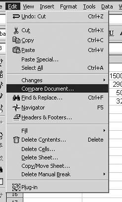
Figure 9.13: The Edit menu.

When we reach the Insert drop-down menu, we begin to get to some really interesting functionality. It is from this menu, shown in Figure 9.14, that you will be able to add new rows, columns, cells, graphics, and more. The addition of rows and columns is relatively straightforward and does not require much explanation. A row or column will be inserted at the spot where your cursor is.

Figure 9.14: The Insert menu.

You also can see the Insert Function option. This will insert the same built-in functions that we examined previously in this chapter. After that you can see the Graphics option. This option will present you with a dialog box, shown in Figure 9.15, where you can insert any standard image file on your machine.

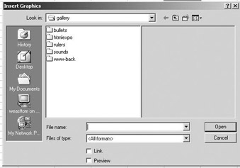
Figure 9.15: Inserting graphics.

Of even more interest is the Insert Object option. This option enables you to insert sounds, videos, OLE objects, Java applets, and more. This enables you to add a whole new dimension to your spreadsheets. For example, if you are doing a budget spreadsheet for a construction project, you could add a video of a building being built. You can do this in Microsoft Excel as well. You simply choose Insert and then select Object. You can then insert video clips, sound files, and more.

Inserting a chart, which you can do in Microsoft Excel, is a very common task in any spreadsheet tools. A spreadsheet is an excellent way to organize data and perform calculations. However, most people respond best to visual cues such as charts. If you select Insert and then choose Chart, you will see a screen, shown in Figure 9.16, that prompts you to choose what cells to include in your chart. You can also select which rows and columns you want to use as labels for your chart.

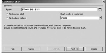
Figure 9.16: The Chart Wizard step one.

The next step, shown in Figure 9.17, enables you to select the various settings for your chart. You can select from bar charts, pie charts, line graphs, and 3D charts. There are a number of options at your disposal. You also can choose whether to display your data in rows or columns. For our purposes we will choose columns and a bar chart, then press Next.

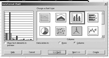
Figure 9.17: The Chart Wizard step two.

The next screen enables you to choose whether you want horizontal (X) and/or vertical (Y) grid lines. You then move to the next screen, shown in Figure 9.18, where you can enter a title for your chart and titles for the X and Y axes.

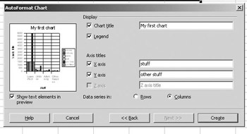
Figure 9.18: The Chart Wizard step three.

When you are done and press the Create button, you will have created a chart, much like the one shown in Figure 9.19. Charts are a very important addition to any spreadsheet. For most people, a chart is required to make the data really come alive.

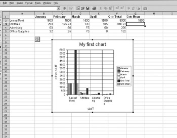
Figure 9.19: Your chart.

You can see that creating a chart is a relatively simple thing to do with Open Office Calc. Charts are a very important part of any spreadsheet application. Storing data, running calculations, and creating charts are the essential elements of any spreadsheet application.

The next button on this toolbar enables you to add simple drawings to your spreadsheet. This may seem like an unnecessary or even frivolous addition to a spreadsheet application, but that is not necessarily correct. The various drawing options, seen in Figure 9.20, enable you to add even more visual impact to your data presentation. When appropriately combined with a chart, this can make the presentation of your data far more compelling than it otherwise would be. Any graphical representation of your data has an important impact on the way others will receive and form conclusions based on that data.

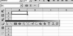
Figure 9.20: The drawing options.

Further down the toolbar we come to an option not present in Microsoft Excel. That option is themes. When you place your mouse over that button, the caption says Choosing Themes. When you click this button, you see the image in Figure 9.21. This enables you to select a theme for your spreadsheet.

Figure 9.21: Open Office Theme Selection.

For example, the Sun theme shown in Figure 9.22 is just one of the several themes you can select. Of course, these themes do not offer any new functionality to your spreadsheet, but just like charts and drawings, themes can add a new dimension to the presentation of your data.

Figure 9.22: The Sun theme.

---