ONS 15454 MSTP Manual DWDM Design Example

When planning and designing DWDM networks, the span losses often are unequal because of such factors as varied optical fiber lengths, differing optical fiber splices/losses, condition of the fiber plant, and so on. In those cases, Tables 10-2, 10-3, and 10-4 serve as a good reference but cannot be used to ensure the operability of the DWDM design. Therefore, the DWDM engineer must manually compute the optical characteristics of each span to measure ONS 15454 MSTP design rule conformity.

This section examines a two-span, linear ONS 15454 MSTP design, using fixed-channel OADMs. Table 10-5 provides the DWDM channel requirements and pertinent design details. Figure 10-3 illustrates the DWDM network requirements.

Table 10-5. ONS 15454 MSTP Network Design Example Requirements

Site Name	DWDM Channel Requirements		Protected (Y/N)	Transponder Type	SFP
	Channel Number	Z Location
Node A	12	Node B	N	DM-L1-xx.x	1310 nm
Node A	34	Node B	N	DM-L1-xx.x	1310 nm
Node A	56	Node B	N	DM-L1-xx.x	1310 nm
Node A	78	Node B	N	DM-L1-xx.x	1310 nm
Node A	910	Node C	N	DM-L1-xx.x	1310 nm
Node A	1112	Node C	N	DM-L1-xx.x	1310 nm
Node A	1314	Node C	N	DM-L1-xx.x	1310 nm
Node A	1516	Node C	N	DM-L1-xx.x	1310 nm

Figure 10-3. ONS 15454 MSTP Network Design Example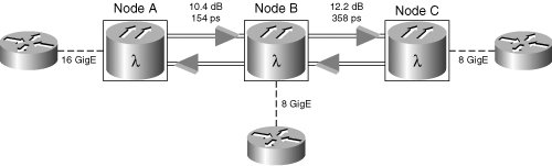

In the next sections, you examine three critical performance aspects of the proposed network:

• Attenuation

• Chromatic dispersion

• OSNR

The sections that follow detail the attenuation from site to site.

Attenuation

Attenuation is the reduction in optical signal power as the fiber pulse travels from one point to another. Consequently, attenuation worsens in direct proportion to the length of optical fiber required for point-to-point transmission. Using optical amplifiers to intermittently energize the optical photons during transmission can mitigate the effects of attenuation. Attenuation can be caused by a combination of natural optical scattering and light-absorption events, such as fiber splices, fiber connectors and terminators, and so on.

Table 10-6 provides the optical attenuation calculations, per span, for the sample network design. This information is helpful in determining whether optical amplifiers are needed and where they should optimally be inserted into the network.

Table 10-6. Optical Attenuation Calculations, Per Span, for Sample Network Design

Node A to Node B (West to East)	Measurement	Comments
Channel input power	+2 dBm	Per-channel power
32-channel multiplexer insertion loss	8.5 dB
Composite signal power	+14 dBm	Power to multiplex 16 channels at +2 dBm per channel
Input power into fiber	7.5 dBm
Fiber plant/splice loss	10.4 dB
Power to Node B	-7.9 dBm
Node B Drop Channels
Input power to OPT-PRE	7.9 dBm
Gain added by OPT-PRE	17.5 dB
Drop loss of 4-channel add/drop filter	5.4 dB
4-channel demultiplex power	11 dBm	Power to demultiplex eight channels at +2 dBm per channel
Channel power to Gigabit Ethernet (GigE) device	1.8 dBm
Node B to Node C (West to East)
Input power to OPT-PRE	2.9 dBm [-5 dBm]	Use input VOA to attenuate to 5 dBm
Gain added by OPT-PRE	17.5 dB
Express power loss from 4-channel add/drop filter	2.5 dB
Input power into fiber	10 dBm
Fiber plant/splice loss	12.2 dB
Input power to OPT-PRE at Node C	2.2d Bm
Gain added by OPT-PRE at Node C	17.5 dB
32-channel demultiplex power	11 dBm	Power to demultiplex 8 channels at +2 dBm per channel
32-channel demultiplexer drop loss	8.5 dB
Channel power to GigE device	4.2 dBm
Node C to Node B (East to West)
Channel input power	+2 dBm	Per-channel power
32-channel multiplexer insertion loss	8.5 dB
Composite signal power	+11 dBm	Power to multiplex 8 channels at +2 dBm per channel
Input power into fiber	4.5 dBm
Fiber plant/splice loss	12.2 dB
Power to Node B	7.7 dBm
Node B to Node A (East to West)
Input power to OPT-PRE	7.7 dBm
Gain added by OPT-PRE	17.5 dB
Express power loss from 4-channel add/drop filter	1.2 dB
Add channels	6.1 dBm	11dBm to multiplex 8 channels4.9 dB channel-insertion loss)
Input power into fiber	14.7 dBm
Fiber plant/splice loss	10.4 dB
Input power to OPT-PRE at Node A	4.3 dBm
Gain added by OPT-PRE at Node C	17.5 dB
32-channel demultiplex power	14 dBm	Power to demultiplex 16 channels at +2 dBm per channel
32-channel demultiplexer drop loss	8.5 dB
Channel power to GigE device	0.7 dBm

Chromatic Dispersion

For DWDM wavelength channels that operate at 2.5 Gbps or below, chromatic dispersion typically does not present a transmission problem. However, in some design cases DWDM wavelength channels operate on aged or deteriorated fiber that could create chromatic dispersion and polarization mode dispersion issues. For the example, the DM-L1-xx.x transponder cards operate with a ±5400 ps/nm chromatic dispersion tolerance. To measure accumulated end-to-end chromatic dispersion, the following formula should be used:

D_link = D_f * L_link

Where:

• D_f is the nominal dispersion of the fiber.

• L_link is the length of the fiber.

In the example, actual chromatic dispersion measurements are given, so compliance measurement is a simple addition operation (that is, 154 ps + 358 ps). With a total chromatic dispersion end-to-end measurement of 512 ps, the network easily fits within the transponder specifications.

OSNR

As an optical signal is cascaded through multiple amplifiers, the signal accumulates noise. If the OSNR at the receiver is less than the interface card specifications, transmissions errors occur. For the example, the DM-L1-xx.x transponder, designed to +5400 ps/nm chromatic dispersion specifications, has an OSNR tolerance of 10 dB. You must calculate the accumulated OSNR to ensure that it is within 10 dB at the terminating optical receiver. Using the OSNR calculation formula given earlier, the following is true:

• The OSNR measurement from Node A to Node B is:

  1 / ([1/630957.3445] + [7.15884 x 10⁹ / 0.000512861]) = 48.1 dB

  Where initial OSNR input is 58 dB (630957.34445 mW)

  Input to OPT-PRE is 2.9 dBm (0.000512861 W)

• The OSNR measurement from Node B to Node C is:

  1 / ([1/64565.4229] + [7.15884 x 10⁹ / 0.00060256]) = 45.6 dB

  Where OSNR input is 48.1 dB (64565.4229 mW)

  Input to OPT-PRE is 2.2 dBm (0.00060256 W)

• The OSNR measurement from Node C to Node B is:

  1 / ([1/630957.3445] + [7.15884 x 10⁹/0.000169824]) = 43.6 dB

  Where initial OSNR input is 58 dB (630957.34445 mW)

  Input to OPT-PRE is 7.7 dBm (0.000169824 W)

• The OSNR measurement from Node B to Node A is:

  1 / ([1/22908.67653] + [7.15884 x 10⁹/0.002691535]) = 43.3 dB

  Where OSNR input is 43.6 dB (22908.67653 mW)

  Input to OPT-PRE is 4.3 dBm (0.002691535 W)

Note

The conversion from decibels to milliwatts is 10E (dBm/10).

As you can see from the example in this section, even the simplest of DWDM designs can involve some degree of complexity. The MSTP DWDM design can become even more complicated when the system transports wavelengths operating at varied bit rates. Each transponder/muxponder type exhibits varying degrees of optical transmit power, OSNR sensitivity, dispersion tolerance, and so on. Manual design of complex systems lends itself to human computational error and can be extremely time-consuming.

To alleviate the design headaches associated with ONS 15454 MSTP networks, Cisco Systems has created a Java-based design tool: MetroPlanner, discussed in the next section.