Section 2.2. Fundamental Link State Concepts
2.2. Fundamental Link State ConceptsTo recap, the two most serious problems with most vector protocols are:
This section looks at the basics of link state routing, with emphasis on how it avoids these two problems. Slow convergence in vector protocols is due to the hop-by-hop, distributed calculation of routes. The more routers on a routethe larger the network isthe longer the convergence time. Suppose that instead of having to perform a route calculation before passing along the results of the calculation, a router could pass an update along to its downstream neighbors as soon as it is received, and then perform its route calculation on a copy of the update afterward? The improvement in convergence time is apparent: Routing information can be sent throughout the routing domain almost as fast as the routers can forward it. Convergence can then happen in all routers at almost the same time. What is the nature of the shared routing information used in such a forward-then-calculate scheme? If the routing information is received and forwarded before a calculation is performed, the information must be independent of the calculation. In other words, each router along a route is performing a local calculation independent of any other router's calculation, and the result of each router's calculation is not shared with other routers. If the calculations are local, it is imperative that all routers along a route derive the same conclusions so that packets are forwarded consistently. Therefore, the information must be exactly the same for each router. No router can alter the information in any way as it is passed along. But the information must be originated somewhere. A route always pertains to some destination address, so it makes sense that the originator of the information is the router directly attached to the destination. It makes sense for another reason, too: If no router is sharing the results of its route calculations with any other router, the only thing it can know before any calculation is itself and its directly connected links.[4]
So, then, the shared information is an announcement[5] by a router identifying itself in some way, and identifying the addresses of the links attached to it.
It is not enough, however, for some router a number of hops away from the destination to receive an announcement of, "I am router A, and I have a directly connected subnet of X." The receiving router must still know how to reach router A. Therefore, every router in the network must send an announcement identifying itself, its links, and the cost associated with each link. One final piece of information must be included in the individual announcements for everything to work properly: Each router must not only identify itself and its directly connected links, but must also identify any directly connected neighboring routers on those links. Neighbors are easily identified if every router transmits messagesHello messageson its links announcing its presence, and listening for Hellos from neighboring routers on the links. As long as the Hellos are never forwarded off of a local link, receiving routers can be sure Hellos are from neighbors. We now have enough details to begin describing a high-level framework for a link state routing protocol:
Figure 2.10 shows how a router might use the database of announcements to determine a route to a destination. The database shown contains the announcements each of the four routers has originated. The announcement from A, for example, shows that it has directly connected links 10.1.1.0 and 10.1.2.0, and a neighbor B. Because all four announcements have been forwarded to all four routers, each of the four routers has a database that looks exactly like the one shown. Figure 2.10. Each router in a link state network has the identical database of routes.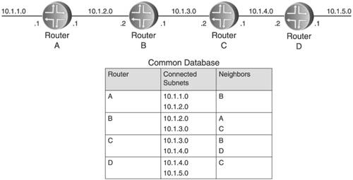 The information in the database is like pieces of a jigsaw puzzle. Without looking at the diagram of the network at the top of Figure 2.10, you can deduce what the network looks like. Router A announced that it has a neighbor B, and B announced that it has a neighbor A. They each are directly connected to subnet 10.1.2.0, so you know that they are connected on this subnet. In the same way, you can look at the announcements of B and C and see that they are connected on subnet 10.1.3.0. Using such deductions, each router can use the database to form a picture of the entire network. From the picture, the router can make entries into its routing table. Router D, for instance, can not only immediately see that subnet 10.1.1.0 is attached to router A, it can see all the routers on the path to A. Therefore, it can make an entry in its database that 10.1.1.0 is reachable via router C, three hops away. This "picture" of the network also reduces the problem of loops. Vector protocols are vulnerable to loops because all a vector protocol router knows about a network is its directly connected links and what its neighbors tell it. But a link state router, because it knows the complete topology of the network, is much less susceptible to these kinds of loops.[6]
Because the routers use the database to maintain state concerning the links and routers in the network, the protocol is called link state. Having described how a link state protocol works at a simplistic level, it is now time to describe the four fundamental concepts of link state protocols. Those concepts are:
2.2.1. AdjacenciesBefore link state routers can begin sending and receiving announcements and building their databases, they must be able to identify their neighbors. And it is not enough to just identify directly connected routers; in some networks, routers might be speaking several routing protocols. A router running a specific link state protocol must be able to find just those directly connected routers running the same protocol. And even this requirement is not good enough. Within the domain of a single routing protocol, there can be constraints on which routers are allowed to exchange route information. So far I have used the term neighbor loosely, but now I will give you a tighter definition: Two routers are neighbors if they should be exchanging route information using a common protocol. If two routers have identified each other as neighbors, each has verified that the other is aware of it, and both have verified that no condition exists that would prevent the exchange of route information,[7] the neighbors are adjacent.
Prerequisite to the operation of a link state protocol is the ability for every router to identify itself. Therefore, each link state router has a router ID (RID), which is an address unique to each router within a single routing domain. The router ID can be administratively assigned, or it can be automatically derived by some means such as using an interface address. The only requirement is that it must be different from the ID used by any other router in the domain, and it must be consistenta router cannot identify itself differently to different neighbors. To identify itself and to discover neighbors, a link state protocol uses Hello messages (an appropriately cheerful name for a protocol used between neighbors). At the least, a Hello message includes the ID of the router that originated the message. The Hello also includes information specific to the routing protocol and relevant to the sending router such as timer settings, interface parameters, and authentication information. Such information is used to ensure, before forming an adjacency, that the two routers are in agreement:
When a routing protocol is enabled on a router, there is usually some method of specifying which connected linksfrom one link to all linksare to be included in the protocol operations. Link state protocols then transmit Hello messages on these links at some regular interval. The messages must be broadcast or multicast, so that any as-yet-undiscovered neighbors will hear them. Because the Hello protocol is used to discover only directly connected neighbors, it is important that no Hello message is ever forwarded beyond the link on which it is transmitted. The originating router can ensure this by methods such as setting the TTL of the IP packet containing the message to 1 or using a multicast address that is specifically scoped to a single link. When a router receives a Hello from a neighbor, it cannot assume that the neighbor has also received its Hellos. If I am router A, and receive Hellos from router B, before I can establish an adjacency I need some indication that B is also receiving my Hellos. Even though I am receiving B's Hellos, it is possible that some sort of half-break in the link is preventing my Hellos from arriving at B. Or, B might be receiving my Hellos and rejecting them for reasons such as packet corruption, incompatible link parameters, or unacceptable protocol parameters within the Hello. Therefore, there must be a procedure by which two-way communication can be verified by both routers. This procedure is called handshaking. An easy way to verify two-way communication is for each router to include in its Hellos on a link a list of all routers from which it has received Hellos on that link. Router A in Figure 2.11 has received a Hello from router B. In its next Hello, A includes B's router ID. When router B receives this Hello, it sees its ID and knows that A is aware of it. Router B responds in kind by including A's ID in its Hellos. When A sees its ID in B's Hellos, it knows B is aware of it. Now both routers have verified two-way communication, and are adjacent. This method of handshaking is called three-way handshaking. Figure 2.11. Three-way handshaking is used to verify two-way communication.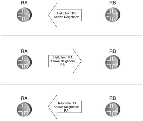 After an adjacency is formed, Hellos serve as keepalives for the adjacency. One of the protocol parameters that a router can include in its Hello messages is a specification of how often it sends Hellos. A receiving router then knows how often to expect Hellos from that neighbor. If the specified time period elapses without the reception of a Hello (allowing some extra time for lost Hellos), a router can assume that the neighbor is no longer active on the link and therefore the adjacency with that neighbor is invalid. Depending on the link state protocol, the Hello period between routers might be predetermined and non-negotiable, the routers might be able to negotiate a Hello period, or the Hello periods of the two routers might be independent (each router just accepts its neighbor's period).
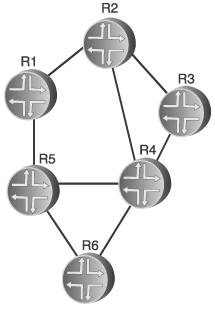
2.2.2. FloodingWithin a network of adjacent routers, each router originates an announcement of its directly connected links and neighbors. As you have already seen, every router in the network must receive every announcement and record a copy in its database. The process of getting the announcement to every router is called flooding. Flooding in the network shown in Figure 2.10 is an easy process: Each router sends its announcement to all of its adjacent neighbors, and each of these neighbors forwards a copy of the announcement to each of its own adjacent neighbors. If split horizon is practiced (no router sends an announcement back to the neighbor it received the announcement from), every router gets a copy of every announcement and the flooding then stops. The network in Figure 2.12 presents more of a challenge for flooding because of all the loops. Just as split horizon rules are insufficient to stop the looping of vector protocol updates in such a topology, split horizon rules are insufficient to control the flooding of link state announcements. A better process is needed to stop the flooding of an announcement after all routers have a copy. Figure 2.12. A well-meshed network poses challenges for flooding. There are other considerations beyond just knowing when to stop flooding. If a router originates an announcement and then fails, how do the other routers know that its announcement no longer is valid? If a router receives differing announcements from the same router, which announcement should be believed? If an announcement becomes corrupted either in transit or in a database, how can a router detect the corruption? Three mechanisms used to create a more reliable flooding process are aging, sequence numbers, and checksums. 2.2.2.1. Timely Flooding: AgingOne of the essential concepts of a link state protocol is that the information in every router's database must be the same as the information in every other router's database. To guarantee "sameness," no router can modify another router's announcement. That means that every router is responsible for its own announcements. What happens, then, if a router fails after flooding an announcement? If the failure is due to a link problem, the neighbors on the link will detect the failure through the Layer 2 protocol. If the failure is a protocol daemon or the router itself, neighbors will detect the failure through the loss of Hello messages. In either case, the effected neighbors send new announcements indicating the change. But now there can be a dilemma. If router A fails, nonadjacent routers receive announcements from A's adjacent neighbors indicating the loss of A. But these routers also still have A's link announcement in their databases. What should be done with those announcements? Can the other routers safely deduce that A has failed and remove A's announcement? Is this a violation of the rule that no router can modify another router's announcement? And more important, how can each router be confident that all other routers have removed the announcement, to preserve database consistency? To help resolve this dilemma, link state protocols include an age field in each link announcement. When a router originates an announcement, it sets a value in the age field. This value is changed (either incremented or decremented)[8] by other routers during flooding, and by every router as the announcement resides in its database. Some absolute value is specified in the protocol at which, if the age reaches this value, the announcement is declared invalid or "aged out," and is deleted from the database. The originating router is responsible for sending a new copy of the announcement at some time prior to this age expiration. The origination of a new announcement is called a refresh. In our example scenario, router A's announcement ages out in all databases because A is no longer refreshing the announcement. Every router in the network then has some assurance that as it deletes A's announcement, all of the other routers are also deleting the announcement.
An age counter can be either up-counting or down-counting. An up-counting age is less flexible because it is set between two absolutes: zero and the maximum age specified in the protocol design. On the other hand, a down-counting age can start at some arbitrary value, bounded at the upper end only by the size of the age field, and counts down to zero. This flexibility has some implication for protocol scalability, and discussed further in Chapter 8. 2.2.2.2. Sequential Flooding: Sequence NumbersWhenever a router receives a link announcement, it sends a copy out each of its downstream interfaces. It is obvious in a well-meshed[9] network such as the one depicted in Figure 2.12 that an announcement will be replicated numerous times during flooding, and as a result some routers will receive multiple copies of the same announcement. If all announcements arrive at the same time, any announcement can be chosen. Of course, delays across different network paths back to the originator are going to vary, so in most cases the multiple copies of the same announcement arrive at different times. In this case, the router might simply accept the announcement with the lowest age, on the grounds that the lowest age indicates the newest announcement.
However, accepting the announcement with the lowest age assumes that the multiple announcements contain the same information. Suppose that very soon after a router originates an announcement a link changes state, prompting a new announcement. It is entirely possible that delay variations in the network could cause the second announcement to arrive with a greater age than the first announcement, causing the second announcement to be incorrectly dropped. Therefore, age is not a reliable determinant for choosing the most recent announcement. A second value, the sequence number, specifies the most recent version of a router's announcement. Given two announcements from the same router, the announcement with the higher sequence number is newer. As with aging, the design of the sequence counter is important. The simplest sequence numbering scheme is a linear one: A sequence number starts at zero, and increments up to some maximum. For example, a 32-bit sequence number (used by both OSPF and IS-IS) can range from zero to 232, or about 4.3 billion. If a router always starts numbering its announcements at sequence number one, this many available numbers should last far beyond the lifetime of the router. Even if a router produces a new announcement every seconda sign of a very unstable linkthe maximum sequence number would not be reached for more than 130 years. Presumably someone would repair the instability before then. What if a router does, for some reason, reach the maximum sequence number? In such a case the router must go back to sequence number 1. The problem is that the last announcement with a high sequence number still resides in databases across the network. If a new announcement is sent with a sequence number of 1, that announcement will be viewed by other routers as an older announcement and will be rejected. To avoid this situation, the router must wait until the existing announcement ages out of all databases. This is unacceptable, because while waiting for the age timer to expirewhich can be one hour or longera possibly incorrect announcement continues to be used for route calculations. There are several possible approaches to this potential problem. One approach is to just do nothing, trusting that with a large enough sequence number space the maximum sequence number will never be reached. The trust here is not that no router or routing protocol is going to remain in uninterrupted service for more than a century, but that no glitches in the protocol daemon will cause the generation of a very high sequence number, introducing the possibility of counting up to the maximum number soon after. A better approach is for the router cycling its sequence numbers back to the beginning to first cause its previous announcement to be deleted from all databases. The router can do this by issuing another copy of the announcement with the maximum sequence number, but with the age set to a value indicating that the announcement's age has expired (MaxAge or 0, depending on whether the age counter is up-counting or down-counting). But remember that when comparing two otherwise identical announcements, the router chooses the one with the lower age. Therefore, the rules must be modified a bit, so that an "aged-out" announcement is always accepted over an identical announcement of any other age. Of course, there is still a period between when the artificially aged-out announcement is sent and the time the new announcement is installed in all databases. Certainly, it is a far smaller period than just waiting for the announcement to age out normally, but it is still a period during which the originating router is not correctly accounted for in the databases. So, a third approach to prevent reaching the end of the sequence number space is to create a space in which there is no end: a circular sequence number space. For example, if there is a 32-bit sequence number space, the number after 4,294,967,295 is 0. However, there is the potential for confusion in this scheme. Suppose two announcements are received from a router, one of which has a sequence number of 0xFFFFFFFC and one with a sequence number of 0xFFF10D69. The sequence numbers are not contiguous; so is the first announcement newer, or has the sequence number wrapped, making the second number higher? A couple of rules can reduce the chance of such confusion. Given some sequence number space of n and two sequence numbers a and b, a is considered larger under either of the following conditions:
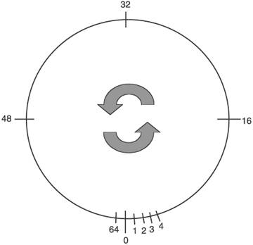
Figure 2.13 shows a diagram of a 6-bit sequence number.[10] A 6-bit space means that
and
Figure 2.13. Sequence numbers in link state protocols could follow a circular number space. Given two sequence numbers 48 and 18, 48 is more recent because by the first rule
Given two sequence numbers 3 and 48, 3 is more recent because by the second rule
Given two sequence numbers 3 and 18, 18 is more recent because by the first rule
You can see by comparing the relative positions of the numbers on the graph in Figure 2.13 how the two rules enforce circularity when there is a discontinuity between two sequence numbers. Although a circular sequence number space seems better than a linear one, an odd series of simultaneous errors in a circular sequence number space can cause a network outage much worse than what sequence number rollover in a linear space causes. This determination is based on a meltdown of the ARPANET on October 27, 1980, when an early link state protocol with a 6-bit circular sequence number space was being used.[11] As a result of that experience, both OSPF and IS-IS use linear sequence numbers.
The last issue with sequence numbers is what happens when a router or protocol restarts and loses all memory of what its last sequence number was. It cannot start again at the beginning, because other routers are likely to have an old announcement from the router in their databases with a higher sequence number, in which case the other routers would reject the new announcement with the lower sequence number. Therefore, another rule is added. When a link state protocol starts, the router sends its announcement with a sequence number of 1 (or whatever the beginning sequence number is for that protocol). If a neighbor has an announcement from the router in its database with a more recent sequence number, it sends a copy of the announcement to the router. The router can then look at the sequence number and begin numbering its new announcements one higher than that number. 2.2.2.3. Reliable Flooding: ChecksumsThe importance of having consistent information in all databases within a link state network has been emphasized throughout this chapter. Yet in networks a link state announcement can become corrupted in many ways. An announcement can be changed due to noise on a link, or it can be corrupted while it resides in a router's database. Because of the possibility of the announcement being altered, there should be a mechanism for checking to ensure that the announcement is accurate. The concern over information corruption certainly extends beyond link state protocols. Most IP packets and messages include error checking, most often in the form of a checksum. A checksum is performed over the entire contents of a link state announcement with the exception of the age field. Because the age changes as the announcement passes through routers during flooding, including it in the checksum would mean recalculating the checksum every time the age changes. 2.2.3. Announcement HeadersWe have now discussed several kinds of identifiers associated with a link state announcement. Some identifiers, such as the router ID, are used to differentiate the announcement from other routers' announcements.[12] Other identifiers, such as the sequence number, age, and checksum, are used to differentiate between specific instances of an announcement from the same router.
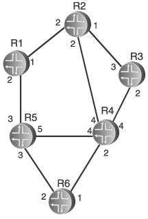
All of these identifiers are included in a header that precedes the actual route information of the announcement. This way, none of the information in the announcement itself must be examined during the flooding processonly the header must be examined. There is also another benefit to having such identifiers in a header. When a router must describe to a neighbor what announcements it has in its database, or when a router must request a copy of an announcement from a neighbor, the announcements can be fully described by sending just the header rather than the entire announcement. Why routers would need to describe announcements to or request announcements from neighbors is explained in the next section. 2.2.4. Database SynchronizationYou should, by now, have a good understanding of a link state database. Announcements from all routers in the network are flooded, and every router keeps a copy of the most recent announcement from every router (including itself) in the database. You also saw how aging is used to ensure that "orphaned" announcements from missing routers are not kept in the database forever. The age of every announcement is tracked, and if the originating router does not refresh the announcement before the age limit is reached, the announcement is deleted from the database. There is one other procedure concerning the link state database that must be explained. When a new link state router becomes active in a network, it floods its announcement to update the other databases. But how does the router build its own database? Requiring the other routers to reflood their announcements when they see a new router's announcement might be one way, but it is not very efficient or scalable. Remember that for a link state protocol to work, every router must have exactly the same database. As you saw in the previous section on flooding, extensive safeguards are implemented to ensure that all databases are identical. This fact can be exploited to allow a new router to build its database without requiring extensive reflooding. After the router forms adjacencies with one or more neighbors, it initiates a database synchronization. When two routers synchronize their databases, they describe the contents of their databases to each other. If a router sees through its neighbor's descriptions that the neighbor has one or more announcements that are not in its own database, the router can request that the neighbor send it a full copy of the announcement. With the assurance that the new router's neighbors have the exact same database as everyone else's, if the router synchronizes with its neighbor it too now has a complete and consistent database. This is where the announcement headers discussed in the preceding section come in. Because an announcement is completely differentiated by its header, only the header needs to be sent during the phases of synchronization in which a neighbor is describing the announcements in its database and when a router is requesting a copy of the announcements it does not have. 2.2.5. SPF CalculationsWith a complete database, the router can begin calculating a shortest path to all other routers in the network. When a path to all routers is known, a path to any of the routers' connected subnets is also known. In the example of Figure 2.10, it was easy to see how the information in a database is used to visualize a network. But it is easy because we are visual creatures. A database describing a more complex topology, such as the one that was shown in Figure 2.12, is not so easy to visualize. But a router's route processor is not visual, it is a computer and thus needs a well-defined set of mathematical rules for calculating shortest paths from the database. This set of rules comes from graph theory and was formulated by Edsger W. Dijkstra. A network is viewed as a graph of nodes, in which the routers are the nodes. Keep in mind that we are calculating shortest paths, so we need some way to assign a cost to each link connecting two nodes. The sum of the costs across a route is the distance of the route. We could, if we wanted, just use router hops. In this case, each link would have a cost of one hop. But router hops limits us in the ways we can define and control traffic patterns in the network. A better scheme is to assign a dimensionless number to each link, as shown in Figure 2.14. Each number then represents the cost of sending a packet out the interface connected to the link. A shortest path is the one in which the total cost of all outgoing interfaces from the source to the destination is the lowest (or "cheapest"). Figure 2.14. A link cost on each path in the network will factor into Dijkstra's algorithm for calculating the shortest-path routing tree in a link state network. We can now influence the choice of shortest paths and, consequently, traffic flows by manipulating the cost of each link. Notice, too, in Figure 2.14 that the costs assigned to the links do not have to be the same at both ends of the links. The costs are assigned to the router interfaces connecting to the links, and apply to outgoing traffic on those interfaces. This way, traffic flows between two routers across the network can be made asymmetric. The clearest description of the Dijkstra algorithm for computing shortest paths in a graph of n nodes comes from Dijkstra himself. Do not worry if the set of rules do not make much sense to you; it will be clearer when we apply it to calculating a shortest-path tree.
Now we can adapt Dijkstra's rules for routers and networks. First, we define the sets. Dijkstra defines three sets of branches: I, II, and III. We define these three sets as follows:
Dijkstra also specifies two sets of nodes, A and B, as follows:
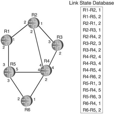
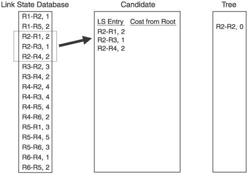
Figure 2.15 shows the network of Figure 2.14 along with the link state database for the network. Each of the entries is in the form [originating router neighbor, cost to neighbor]. The way to read this database is, for instance, that router R1 has sent an announcement indicating two neighbors: neighbor R2, at a cost of 1, and R5, at a cost of 2. R2 has announced three neighbors: R1 with a cost of 2, R3 with a cost of 1, and R4 with a cost of 2. Comparing the entries in the database with the diagram of the network, you can see that all adjacencies are accounted for from the perspective of all routers. Figure 2.15. The link state database includes all router adjacenies and a cost for each. Each router then creates a tree database and a candidate database, and performs the following steps:
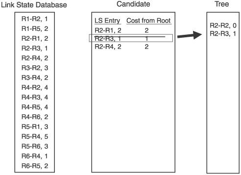
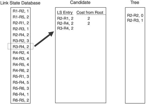
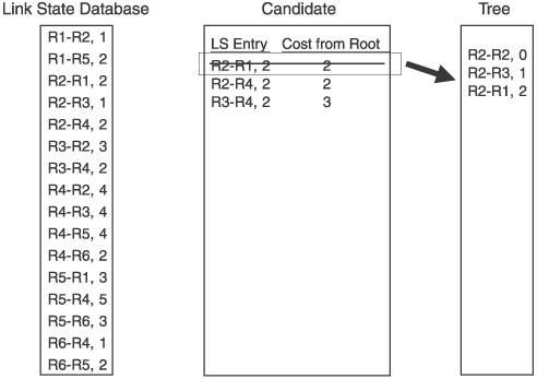
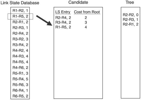
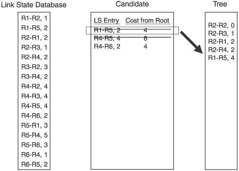
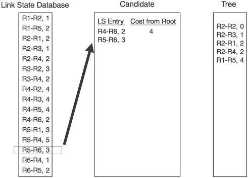
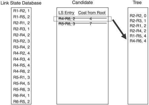
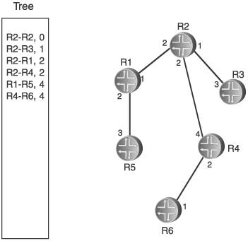
For the example network in Figure 2.15, we focus on the Dijkstra calculation that R2 would perform. Figure 2.16 shows the link state database from Figure 2.15, along with the candidate and tree databases. R2 has added itself to the tree as the root, with a cost of 0, completing Step 1. R2 then looks into its link state database for all links to neighbors, and adds those to the candidate database. R2's neighbors are R1, R3, and R4, so these three entries are added to the candidate list. This completes Step 2. Figure 2.16. R2 begins building its shortest-path tree. Figure 2.17 shows the completion of the first iteration of Step 3. The cost from the root to each of the neighbors on the link is calculated. In this case, because the neighbors are directly connected, the cost is just the cost of the link. The entry with the lowest cost from the root is then selected, which in this case is the link to R3. This entry is moved from the candidate list to the tree. Figure 2.17. When the entry with the lowest path is added to the tree, it is removed from the candidate list. Step 4 is performed in Figure 2.18. Because the link to R3 was added to the tree in the preceding step, all of the entries in the database showing links to R3's neighbors are examined. R3 has links to R2 and to R4. Because a link to R2 is already in the database, that entry is ignored. Only the link to R4 is added to the candidate list. Figure 2.18. R3's path to R4 is added to the candidate database; R3's path to R2 is ignored because a path to R2 already exists in the tree. Step 5 says that if there are entries in the candidate database, return to Step 3. So, Step 3 is repeated in Figure 2.19. The cost from the root to the neighbor in the new entry is calculated, which is the cost of the link from R2 to R3, shown in the tree database to be 1, and the cost from R3 to R4, which is 2, for a total of 3. The lowest cost from the root in the candidate database is then selected. This time, there are two lowest costs: R2-R1, and R2-R4. Step 3 says that if two or more costs are equal, just select one. So we select R2-R1 and move it from the candidate list to the tree. Figure 2.19. When there are two or more lowest cost entries in the candidate database, pick one to move to the tree database. Figure 2.20 shows the second iteration of Step 4. R1 was added to the tree in the previous step, so the link state database entries for R1's neighbors, R1-R2 and R1-R5, are examined. R2 is already on the tree, so only the R1-R5 entry is added to the candidate list. Figure 2.20. R1's path to R5 is added to the candidate database. R1's path to R2 is ignored because a path to R2 already exists in the tree. We cycle back to Step 3 again in Figure 2.21. The cost from the root to R5 is 4, which is the cost from R2 to R1 plus the cost from R1 to R5. The costs from root are again examined, R2-R4 is found to have the lowest cost, and it is moved from the candidate list to the tree. Because the shortest path to R4 is now on the tree, the longer R3-R4 link on the candidate list is removed from the candidate list. Figure 2.21. The cost from the root to R5 is the cost of R2 to R1 (2) plus the cost of R2 to R5 (2). R4's four entries in the database are examined next. R2 and R3 are already on the tree, so only the entries for links from R4 to R5 and R6 are added to the candidate list. Figure 2.22. R4's paths to R4 and R5 are added to the candidate database. R4's paths to R2 and R3 are ignored because paths to R2 and R3 already exist in the tree. Costs to the root are again calculated. The cost to R5 through R4 is 6 (R2-R4 plus R4-R5), and the cost to R6 through R4 is 4 (R2-R4 plus R4-R6). There are two entries with a low cost of R4, so we arbitrarily choose the R1-R5 entry and move it to the tree. There is a longer link to R5 via R4 on the candidate list, so this entry is removed. Back to Step 3 again in Figure 2.24. The only entry from R5 that does not have a neighbor that is already on the tree is R5-R6, so this one entry is added to the candidate list. Figure 2.23. Choose one of the two lowest-cost paths to move to the tree. Delete the longer path from the root to R5 from the candidate database. Figure 2.24. Of R5's neighbors, only R6 is not yet on the tree, so add R5-R6 to the candidate database. In Figure 2.25 the cost from the root to R6 through R5 is 7 (R1-R5 plus R5-R6). The R4-R6 entry, with a cost of 4, is moved to the tree. And because R6 is now on the tree, the R5-R6 entry is removed from the candidate list. At this time, when we go to Step 4, we find that there are no entries in the link state database from R6 that lead to a neighbor that is not already on the tree. Therefore, the candidate list is empty, which Step 5 says is the indication that the computation is complete. Figure 2.25. From the candidate database, add the smaller cost path to the tree and delete R5-R6 because a shorter path already exists in the tree. The tree database now describes the shortest path from R2 to every other router in the network. Figure 2.26 shows the tree database and the network diagram, with only the links of the tree showing. Figure 2.26. The shortest path from the node (R2) to each other router in the network now resides in the tree database. An important detail of the calculation that was just performed has to do with loops. The tree from the rootthe router doing the calculationis built branch by branch, and at no point during the calculation was there a loop on the tree. This is because no entry is added to the tree that has a neighbor already on the tree, and any entry on the candidate list that has a neighbor already on the tree is removed from the list before the next iteration of the calculation is performed. This is a major advantage of link state protocols over vector protocols using a Bellman-Ford algorithm: There is no point during this calculation when loops might occur. Link state protocols are therefore more stable in times of network transition. 2.2.6. AreasIf a link state network grows very large, the flooding procedures and the link state database can begin presenting scaling problems. Flooding is a problem because as more routers are added to the network, announcement refresh activity becomes more and more frequent. Although the refresh interval is set by protocol parameters, the times at which each router's refresh timer expires are randomly distributed throughout the network. This is a good thing. You would not want all routers' refresh timers expiring at the same time, creating a massive flood of announcements and a corresponding spike in traffic and processing load. The link state database can become a scalability problem in large networks because all announcements from all routers must be stored and then used in the Dijkstra SPF calculation. I took a long time and much page space to describe the Dijkstra calculation in the preceding section, but a router can perform the calculations extremely fast. But if the number of entries in the link state database is in the thousands rather than in the tens or hundreds, the corresponding SPF calculations might become burdensome. Another factor in the scalability of link state protocols is the fact that all routers in the network must maintain and process exactly the same database as every other router. So, if you have a network built with dozens of high-memory, high-powered core routers and one low-memory, low-powered router, the performance of your entire network is bounded by the capabilities of this one small router. These basic link state scaling problems are countered by breaking up the network into areas. With areas, the database and flooding rules are modified as follows:
Some routers must connect areas, and are called (in OSPF, anyway) area border routers. The modified link state database rule says that all routers within an area must have the same link state database, so area border routers must maintain separate link state databases for each area to which they are attached. The scope of the trees calculated by the routers internal to an area is the area boundary. Area border routers calculate multiple trees, one for each of its attached areas. The entire reason for flooding is to ensure that all link state databases have the same entries. If the databases must now only be identical within an area, the scope of flooding is also defined by the area boundaries.[14] Area border routers know all destinations within an attached area, and send an announcement into its other attached areas listing these destinations. So rather than have all announcements from the routers in an area flooded throughout a routing domain, the area is represented by a single announcement from each of its border routers. Areas also help reduce the problem of one router imposing limitations on the entire domain. Small, low-powered routers can be placed in small areas, thereby keeping the link state database size and flooding traffic well within the capabilities of the small routers.
|


EAN: 2147483647
Pages: 111