Swept Surfaces

Implementing NURBS in Code

As I mentioned at the beginning of the chapter, the bulk of conceptual and implementation work for NURBS was done in the previous chapter. Therefore, I'm only going to give the new snippets here in the text. The full source code is available in the \Code\Chapter05 directories on the CD.

In NURBSApplication.h, you will see that the class has been augmented with several members that handle the weighting factors and new basis functions. As with all the source code, there are probably ways to make this code more efficient and less memory intensive , but this format is very clear. Note that the following code only includes the additions to the code.

The first additions are a weight vector and a function to set the weight values. This is very analogous to the knot vector and setting function seen in the previous chapter.

 float m_Weights[NUM_CONTROL_POINTS]; void  SetWeights(); 

Next, I have added separate arrays for the weighted basis functions. You could limit the amount of memory used by folding the B-spline arrays and NURBS arrays together or by allocating only enough memory for the final order, but I have created a full duplicate in case you want to compare the basis functions.

 float m_NURBSBasisFunctions[NUM_CURVE_VERTICES]                            [NUM_CONTROL_POINTS]                            [CURVE_ORDER]; float m_NURBSDerivativeBasis[NUM_CURVE_VERTICES]                             [NUM_CONTROL_POINTS]                             [CURVE_ORDER]; 

The weight vector is filled with the SetWeights function found in NURBSApplication.cpp. I have set up this function so that each weight is first set to 1.0. After that, you can individually set the weights of different control points as you see fit. The following code creates an animated weight for the third control point.

 void CNURBSApplication::SetWeights() {        for (long i = 0; i < NUM_CONTROL_POINTS; i++)               m_Weights[i] = 1.0f;        m_Weights[2] = 10.0f * fabs(sin((float)GetTickCount() / 2000.0f)); } 

Next comes the real meat of the code. The DefineBasisFunctions function has been augmented to create NURBS basis functions based on the B-spline functions seen in the last chapter. The function creates the array of B-spline basis values just as it did for the previous chapter, but it now includes one final step where the irrational basis functions, the weight vector, and Equations 5.1 and 5.3 are used to generate the NURBS basis functions and their derivatives. Again, you probably will only need the highest-order values, but I loop through all the orders here for the sake of completeness.

 for (Order = 1; Order < CURVE_ORDER; Order++) {        for (long ControlPoint = 0; ControlPoint < NUM_CONTROL_POINTS;             ControlPoint++)        {               for (long Vertex = 0; Vertex < NUM_CURVE_VERTICES;                    Vertex++)               { 

As you loop through each order, control point, and parameter value, you can find the NURBS basis functions using Equations 5.1 and 5.3. The denominator of the basis function and the numerator of the second term of Equation 5.3 are both based on the sums of the products of the weights and irrational basis functions. Before computing the rational functions, you must first find those sums by looping through the irrational functions and multiplying them by the values in the weight vector.

 float Denominator = 0.0f;                 float SumDerivatives = 0.0f;                 for (long ControlWeight = 0;                      ControlWeight < NUM_CONTROL_POINTS; ControlWeight++)                 {                        Denominator += m_Weights[ControlWeight] *                                       m_BasisFunctions[Vertex]                                      [ControlWeight][Order];                        SumDerivatives += m_Weights[ControlWeight] *                                          m_DerivativeBasis[Vertex]                                          [ControlWeight][Order];                 } 

Now that you have those sums, you can assemble the rational basis functions for both the curve and the derivative. The following code is the C++ implementation of Equations 5.1 and 5.3.

 m_NURBSBasisFunctions[Vertex][ControlPoint][Order] =                    m_Weights[ControlPoint] *                    m_BasisFunctions[Vertex][ControlPoint][Order] /                    Denominator;                 m_NURBSDerivativeBasis[Vertex][ControlPoint][Order] =                    (m_Weights[ControlPoint] *                    m_DerivativeBasis[Vertex][ControlPoint][Order] /                    Denominator) -                   (m_Weights[ControlPoint] *                    m_BasisFunctions[Vertex][ControlPoint][Order] *                    SumDerivatives / (Denominator * Denominator));                 }        } } 

Figure 5.17 shows a screenshot from the application found in the \Code\Chapter05 - NURBS with Open Uniform Knot Vector directory. I have enabled the basis function drawing functionality ( DrawBasisFunctions now draws the NURBS values).

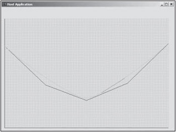
Figure 5.17: Screenshot of basic NURBS application.

I have also supplied two projects for drawing conic sections. The first one is very basic. It uses the preceding code, only this time the knot vector, weights, and control points are set to draw a circle with a triangle, as shown in Figure 5.11. The following snippets of code can be found in the \Code\Chapter05 - NURBS Conic Section 1 directory.

First, set the weights to match the values needed for a 120 degree arc.

 void CNURBSApplication::SetWeights() {        for (long i = 0; i < NUM_CONTROL_POINTS; i++)               m_Weights[i] = 1.0f;        m_Weights[1] = m_Weights[3] = m_Weights[5] = 0.5f; } 

Now, set the knot vector needed to concatenate the three arcs.

 void CNURBSApplication::SetKnotVector() {        m_KnotVector[0] = m_KnotVector[1] = m_KnotVector[2] = 0.0f;        m_KnotVector[3] = m_KnotVector[4] = 0.333f;        m_KnotVector[5] = m_KnotVector[6] = 0.666f;        m_KnotVector[7] = m_KnotVector[8] = m_KnotVector[9] = 1.0f; } 

Finally, set the locations of the control points to draw a control polygon in the shape of an equilateral triangle. This code can be found in the DefineBasisFunctions function.

 for (long ControlPoint = 0; ControlPoint < NUM_CONTROL_POINTS; ControlPoint++) {        pVertices[ControlPoint].z = 1.0f;        pVertices[ControlPoint].color = 0xFF000000; } pVertices[0].x = 300.0f; pVertices[0].y = 0.0f; pVertices[1].x = 500.0f; pVertices[1].y = 0.0f; pVertices[2].x = 400.0f; pVertices[2].y = 173.0f; pVertices[3].x = 300.0f; pVertices[3].y = 346.0f; pVertices[4].x = 200.0f; pVertices[4].y = 173.0f; pVertices[5].x = 100.0f; pVertices[5].y = 0.0f; pVertices[6].x = 300.0f; pVertices[6].y = 0.0f; 

Figure 5.18 is a screenshot from this application including the basis functions.

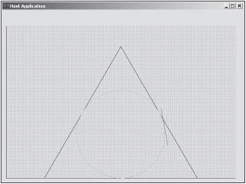
Figure 5.18: Screenshot of basic conic section application.

This application was built with hardcoded values so that you could easily see the way a simple circle was built. The code found in \Code\Chapter05 - NURBS Conic Section 2 uses Equation 5.2 and the concepts from Figure 5.12 to create circles with an arbitrary? number of sides.

First, the weights are set. The odd control points represent the apex of each of the triangular subsections, so they must be weighted according to Equation 5.2. The even control points are given a weight of 1.0.

 void CNURBSApplication::SetWeights() {        for (long i = 0; i < NUM_CONTROL_POINTS; i++)        {               if (i % 2)                      m_Weights[i] = cos(TWO_PI / (float)NUM_SIDES / 2.0f);               else                      m_Weights[i] = 1.0f;        } } 

Next, the concatenated knot vector is created. It is a nonuniform open knot vector created using the rationale seen in Figure 5.15.

 void CNURBSApplication::SetKnotVector() {        m_KnotVector[0] = m_KnotVector[1] = m_KnotVector[2] = 0.0f;        for (long i = 3; i < CURVE_ORDER + NUM_CONTROL_POINTS - 3; i += 2)        {               m_KnotVector[i] = m_KnotVector[i + 1] =                              (((float)i - 1.0f) / 2.0f) /                              (float)NUM_SIDES;        }        m_KnotVector[i] = m_KnotVector[i + 1] = m_KnotVector[i + 2] = 1.0f; } 

Finally, the control points are set following the rationale shown in Figure 5.12. The even points lie on the inscribed circle; the odd points lie on the circumscribed polygon.

 for (long ControlPoint = 0; ControlPoint < NUM_CONTROL_POINTS; ControlPoint++) {        float Radius;        if (ControlPoint % 2)               Radius = 100.0f / cos(TWO_PI / (2.0f * (float)NUM_SIDES));        else               Radius = 100.0f;        pVertices[ControlPoint].x = 300.0f + Radius *                                    cos((float)ControlPoint * TWO_PI /                                        (2.0f * (float)NUM_SIDES));        pVertices[ControlPoint].y = 200.0f + Radius *                                    sin((float)ControlPoint * TWO_PI /                                        (2.0f * (float)NUM_SIDES));        pVertices[ControlPoint].z = 1.0f;        pVertices[ControlPoint].color = 0xFF000000; } 

Figure 5.19 shows a screenshot of a circle formed with an octagonal control polygon. As the number of control points increases , you have more freedom to create shapes such as those seen in Figure 5.14.

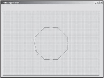
Figure 5.19: Circle from an octagonal control polygon.