Rhino 2.0 (Evaluation Version)

 

Introducing the Curve Application

Each chapter will include code that highlights the more important points of the chapter. I have chosen to make the applications very simple so that you can concentrate on the curve concepts rather than the details of rendering. That said, I will spend very little time talking about the specifics of rendering in order to save space. The code is written in DirectX, but it should be easy to re-create in OpenGL if you would rather do that. Remember that this code is written to highlight the curves and, therefore, it is not optimized at all.

The source code for this chapter can be found on the CD in the \Code\Chapter01 directory. Several of the files in that directory are for the basic framework and can be ignored if you would like (the framework is described in detail in Real-Time Rendering Tricks and Techniques in DirectX , Premier Press, ISBN 1-931841-27-6). Each application includes a base class that handles drawing the basic environment. It sets up the drawing canvas by drawing a grid of lines and a set of axes. It is important to note that the units for drawing the curve are in pixels. This will make things easier in later chapters, but for now it can be a hindrance because some polynomial functions will produce results that quickly move outside the bounds of the application window. To see what I mean, take a look at  CurveApplication.cpp . This is the file that contains all of the chapter-specific code.

The code in  CurveApplication.cpp is very simple. It is meant to introduce you to the application framework with the minimum of distractions and to illustrate the first derivative of polynomial functions. Figure 1.10 shows a screenshot of the application.

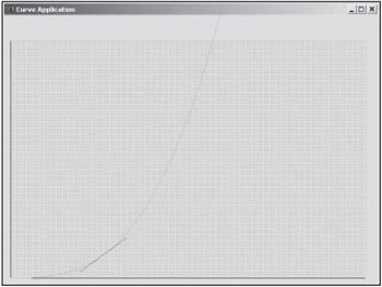
Figure 1.10: A screenshot showing a sample curve and the slope at a given point.

This first application draws a curve and also shows the slope at every point along the curve. You can set the function by redefining this macro at the top of the file.

 #define FUNCTION_X(x) (0.00001f * (float)x * (float)x * (float)x) 

In this case, the y values along the graph are equal to x cubed. I have multiplied it by a very small constant to keep the graph more reasonable. Try removing this constant. You'll see that the curve becomes so steep that it's not even worth looking at.

In this sample, you must specify the first derivative yourself. Do this by setting the second macro.

 #define DERIVATIVE_X(x) (0.00003f * (float)x * (float)x) 

Remember that you must include the scaling constant in the derivative as well. Feel free to experiment with different polynomial functions, but remember to include a scaling factor in all of your calculations.

Once the functions have been set, the application creates the vertices for the actual curve using the following code. The resolution of the curve defines how many points are created. A larger number for the resolution creates more spacing between the points, forming a lower resolution curve.

 int Index = 0;         for (int x = 0; x <= 600; x += CURVE_RESOLUTION)         {                pVertices[Index].x     = (float)x;                pVertices[Index].y     = FUNCTION_X((float)x);                pVertices[Index].z     = 1.0f;                pVertices[Index].color = 0xFFFF0000;                Index ++;         } 

Figure 1.11 shows a lower resolution version of the same curve.

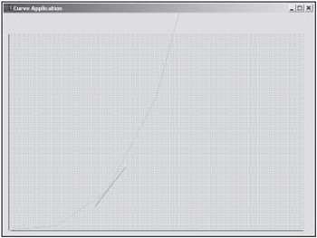
Figure 1.11: A lower resolution version of the curve in Figure 1.10.

The application uses these vertices to draw the curve every frame. In addition, the application also draws an animated slope line at the different points along the curve. It does this by setting the positions of two points using the following code. The current x value is based on the current system time. The modulo operator keeps the x position within the valid x range, but the result may still appear offscreen .

 float CurrentX = (float)((GetTickCount() / 10) % 600); 

The rest of the code includes a fair amount of trigonometry, which leads very well into the next chapter. This code uses arctangent to find the angle of the slope and then uses the angle value to figure out x and y positions with the help of the current position on the curve and the length of the slope line. Once these positions are computed, the application will draw the slope line.

 float CurrentSlope = DERIVATIVE_X(CurrentX);        float CurrentAngle = atan(CurrentSlope);        pVertices[0].x = CurrentX + SLOPE_WIDTH * cos(CurrentAngle);        pVertices[0].y = FUNCTION_X(CurrentX) + SLOPE_WIDTH * sin(CurrentAngle);        pVertices[0].z     = 1.0f;        pVertices[0].color = 0xFF0000FF;        pVertices[1].x = CurrentX - SLOPE_WIDTH * cos(CurrentAngle);        pVertices[1].y = FUNCTION_X(CurrentX) - SLOPE_WIDTH * sin(CurrentAngle);        pVertices[1].z     = 1.0f;        pVertices[1].color = 0xFF0000FF; 

Obviously, I have breezed past much of the code in this first application. The code will be very simple if you've worked with DirectX before. If not, take some time to experiment with the code before moving on. The rest of the chapters are based on the same basic ideas and framework.