Other Search Expressions

In addition to the SELECT statement and joins, SQL Server provides other useful search expressions that enable you to tailor your queries. These expressions include LIKE and BETWEEN, along with aggregate functions such as AVG, COUNT, and MAX.

LIKE

In an earlier example, we used LIKE to find authors whose names start with Ri. LIKE allows you to search using the simple pattern matching that is standard with ANSI SQL, but SQL Server adds capability by introducing wildcard characters that allow the use of regular expressions. Table 7-4 shows how wildcard characters are used in searches.

Table 7-4. Wildcard characters recognized by SQL Server for use in regular expressions.

Wildcard	Searches for
%	Any string of zero or more characters.
_	Any single character.
[ ]	Any single character within the specified range (for example, [a-f]) or the specified set (for example, [abcdef]).
[^]	Any single character not within the specified range (for example, [^a-f]) or the specified set (for example, [^abcdef]).

Table 7-5 shows examples from the SQL Server documentation of how LIKE can be used.

Table 7-5. Using LIKE in searches.

Form	Searches for
LIKE 'Mc?%'	All names that begin with the letters Mc (such as McBadden).
LIKE '?%inger'	All names that end with inger (such as Ringer and Stringer).
LIKE '?%en?%'	All names that include the letters en (such as Bennet, Green, and McBadden).
LIKE '_heryl'	All six-letter names ending with heryl (such as Cheryl and Sheryl).
LIKE '[CK]ars[eo]n'	All names that begin with C or K, then ars, then e or o, and end with n (such as Carsen, Karsen, Carson, and Karson).
LIKE '[M-Z]inger'	All names ending with inger that begin with any single letter from M through Z (such as Ringer).
LIKE 'M[^c]%'	All names beginning with the letter M that don't have the letter c as the second letter (such as MacFeather).

Trailing Blanks

Trailing blanks (blank spaces) can cause considerable confusion and errors. In SQL Server, when you use trailing blanks you must be aware of differences in how varchar and char data is stored and of how the SET ANSI_PADDING option is used.

Suppose that I create a table with five columns and insert data as follows:

 SET ANSI_PADDING OFF DROP TABLE checkpad GO CREATE TABLE checkpad ( rowid smallint NOT NULL PRIMARY KEY, c10not char(10) NOT NULL, c10nul char(10) NULL, v10not varchar(10) NOT NULL, v10nul varchar(10) NULL ) -- Row 1 has names with no trailing blanks INSERT checkpad VALUES (1, 'John', 'John', 'John', 'John') -- Row 2 has each name inserted with three trailing blanks INSERT checkpad VALUES (2, 'John ', 'John ', 'John ', 'John ') -- Row 3 has each name inserted with a full six trailing blanks INSERT checkpad VALUES (3, 'John ', 'John ', 'John ', 'John ') -- Row 4 has each name inserted with seven trailing blanks (too many) INSERT checkpad VALUES (4, 'John ', 'John ', 'John ', 'John ') 

I can then use the following query to analyze the contents of the table. I use the DATALENGTH(expression) function to determine the actual length of the data and then convert to VARBINARY to display the hexadecimal values of the characters stored. (For those of you who don't have the ASCII chart memorized, a blank space is 0x20.) I then use a LIKE to try to match each column, once with one trailing blank and once with six trailing blanks.

 SELECT ROWID, "0xC10NOT"=CONVERT(VARBINARY(10), c10not), L1=DATALENGTH(c10not), "LIKE 'John %'"=CASE WHEN (c10not LIKE 'John %') THEN 1 ELSE 0 END, "LIKE 'John %'"=CASE WHEN (c10not LIKE 'John %') THEN 1 ELSE 0 END, "0xC10NUL"=CONVERT(VARBINARY(10), c10nul), L2=DATALENGTH(c10nul), "LIKE 'John %'"=CASE WHEN (c10nul LIKE 'John %') THEN 1 ELSE 0 END, "LIKE 'John %'"=CASE WHEN (c10nul LIKE 'John %') THEN 1 ELSE 0 END, "0xV10NOT"=CONVERT(VARBINARY(10), v10not), L3=DATALENGTH(v10not), "LIKE 'John %'"=CASE WHEN (v10not LIKE 'John %') THEN 1 ELSE 0 END, "LIKE 'John %'"=CASE WHEN (v10not LIKE 'John %') THEN 1 ELSE 0 END, "0xV10NUL"=CONVERT(VARBINARY(10), v10nul), L4=DATALENGTH(v10nul), "LIKE 'John %'"=CASE WHEN (v10nul LIKE 'John %') THEN 1 ELSE 0 END, "LIKE 'John %'"=CASE WHEN (v10nul LIKE 'John %') THEN 1 ELSE 0 END FROM checkpad 

Figure 7-2 shows the results of this query from the checkpad table.

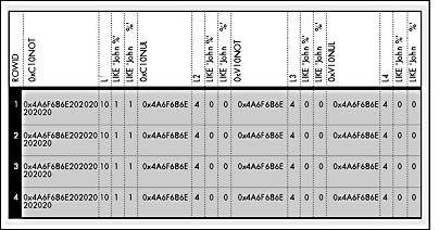
Figure 7-2. The results of the query using SET ANSI_PADDING OFF.

If you don't enable SET ANSI_PADDING ON, SQL Server trims trailing blanks for variable-length columns and for fixed-length columns that allow NULLs. Notice that only column c10not has a length of 10. The other three columns are treated identically and end up with a length of 4 and no padding. For these columns, even trailing blanks explicitly entered within the quotation marks are trimmed. All the variable-length columns as well as the fixed-length column that allows NULLs have only the 4 bytes J-O-H-N (4A-6F-68-6E) stored. The true fixed-length column, c10not, is automatically padded with six blank spaces (0x20) to fill the entire 10 bytes.

All four columns match LIKE 'John%' (no trailing blanks), but only the fixed-length column c10not matches LIKE 'John ?' (one trailing blank) and LIKE 'JOHN %'?' (six trailing blanks). The reason is apparent when you realize that those trailing blanks are truncated and aren't part of the stored values for the other columns. A column query gets a hit with LIKE and trailing blanks only when the trailing blanks are stored. In this example, only the c10not column stores trailing blanks, so that's where the hit occurs.

SQL Server has dealt with trailing blanks in this way for a long time. However, when the developers began working to pass the National Institute of Standards and Technology (NIST) test suite for ANSI SQL conformance, they realized that this behavior was inconsistent with the ANSI specification. The specification requires that you always pad char datatypes and that you don't truncate trailing blanks entered by the user, even for varchar. I could argue for either side—both the long-standing SQL Server behavior and the ANSI specification behavior can be desirable, depending on the circumstances. However, if SQL Server had changed its behavior to conform to ANSI, it would have broken many deployed SQL Server applications. So, to satisfy both sides, the ANSI_PADDING option was added in version 6.5. If you enable SET ANSI_PADDING ON, re-create the table, reinsert the rows, and then issue the same query, you get the results shown in Figure 7-3, which are different from those shown in Figure 7-2.

If you set ANSI_PADDING ON, the char(10) columns c10not and c10nul, whether declared NOT NULL or NULL, are always padded out to 10 characters regardless of how many trailing blanks were entered. In addition, the variable-length columns v10not and v10nul contain the number of trailing blanks that were inserted. Trailing blanks are not truncated. Because the variable-length columns now store any trailing blanks that were part of the INSERT (or UPDATE) statement, the columns get hits in queries with LIKE and trailing blanks if the query finds that number of trailing blanks (or more) in the columns' contents. Notice that no error occurs as a result of inserting a column with seven (instead of six) trailing blanks. The final trailing blank simply gets truncated. If you want a warning message to appear in such cases, you can use SET ANSI_WARNINGS ON.

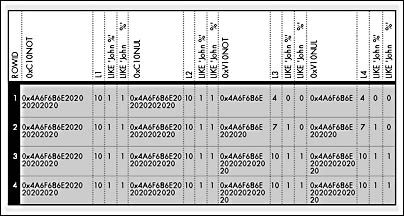
Figure 7-3. The results of the query using SET ANSI_PADDING ON.

Note that the SET ANSI_PADDING ON option applies to a table only if the option was enabled at the time the table was created. (SET ANSI_PADDING ON also applies to a column if the option was enabled at the time the column was added via ALTER TABLE.) Enabling this option for an existing table does nothing. To determine whether a column has ANSI_PADDING set to ON, examine the status field of the syscolumns table and do a bitwise AND 20 (decimal). If the bit is on, you know the column was created with the option enabled. For example:

 SELECT name, 'Padding On'=CASE WHEN status & 20 <> 0 THEN 'YES' ELSE 'NO' END FROM syscolumns WHERE id=OBJECT_ID('checkpad') AND name='v10not' GO 

SET ANSI_PADDING ON also affects the behavior of binary and varbinary fields, but the padding is done with zeros instead of spaces. Table 7-6 shows the effects of the SET ANSI_PADDING setting when values are inserted into columns with char, varchar, binary, and varbinary data types.

Note that when a fixed-length column allows NULLs, it mimics the behavior of variable-length columns if ANSI_PADDING is off. If ANSI_PADDING is on, fixed-length columns that allow NULLs behave the same as fixed-length columns that don't allow NULLs.

The fact that a fixed-length character column that allows NULLs is treated as a variable-length column does not affect how the data is actually stored on the page. If you use the DBCC PAGE command (as discussed in Chapter 6) to look at the column c10nul, you'll see that it always holds a full 10 characters, including the 6 trailing spaces in our example above. When you manipulate the column using SQL statements, the query processor checks the status of the bit in syscolumns.status, and if the column is marked with ANSI_PADDING set to ON, the query processor ignores trailing blanks.

You should also be aware that comparing these strings using LIKE is quite a bit different than comparing the strings for equality. The following query returns only rows in which the query processor recognizes at least one trailing space after the 'John':

 SELECT * FROM checkpad WHERE c10nul LIKE 'John %' 

On the other hand, a comparison that looks for equality always ignores any trailing spaces and finds a match whenever all the leading, nonspace characters are the same. The following query returns all the rows in the checkpad table, whether ANSI_PADDING is ON or OFF, and in addition, it returns all the rows in the table if you replace the c10nul column with any of the columns in the table:

 SELECT * from checkpad WHERE c10nul = 'John' 

The SQL Server ODBC driver and OLE DB Provider for SQL Server automatically set ANSI_PADDING to ON when they connect. When you write your own applications, the ANSI_PADDING setting can be changed in the ODBC connection attributes or the OLE DB connection properties before your application makes its connection to the SQL Server. In addition, the ANSI_PADDING setting can be changed in the ODBC Data Sources dialog box, available through the Control Panel.

Table 7-6. The effects of the ANSI_PADDING setting.

Setting of ANSI_PADDING	char(n) NOT NULL or binary(n) NOT NULL	char(n) NULL or binary(n) NULL	varchar(n) or varbinary(n)
ON	Pad original value to the length of the column.	Follows same rules as for char(n) or binary(n) NOT NULL.	Trailing blanks (for varchar) or zeros (for varbinary) in values inserted aren't trimmed. Values are not padded to the length of the column.
OFF	Pad original value to the length of the column.	Follows same rules as for varchar or varbinary.	Trailing blanks (for varchar) or trailing zeros (for varbinary) are trimmed.

Regardless of how the column was created, SQL Server provides functions that can help you deal effectively with trailing blanks. The RTRIM(char_expression) function removes trailing blanks if they exist. You can add trailing blanks to your output by concatenating with the SPACE(integer_expression) function. An easier way is to use the CONVERT function to convert to a fixed-length char of whatever length you want. Then variable-length columns will be returned as fully padded, regardless of the ANSI_PADDING setting and regardless of the columns' actual storage, by converting them to char(10) or whatever size you want. The following SELECT statement against the checkpad table illustrates this:

 SELECT CONVERT(VARBINARY(10), CONVERT(char(10), v10nul)) FROM checkpad 

Here's the result:

 0x4a6f686e202020202020 0x4a6f686e202020202020 0x4a6f686e202020202020 0x4a6f686e202020202020 

BETWEEN

BETWEEN is shorthand for greater-than-or-equal-to AND less-than-or-equal-to. The clause WHERE C BETWEEN B AND D is equivalent to WHERE C >= B AND C <= D. The order of the values to be checked is important when you use BETWEEN. If B, C, and D are increasing values, for example, WHERE C BETWEEN D AND B isn't true because it evaluates to WHERE C >= D AND C <= B.

Aggregate Functions

Aggregate functions (sometimes referred to as set functions) allow you to summarize a column of output. SQL Server provides six general aggregate functions that are standard ANSI SQL-92 fare. I won't go into much detail about their general use; instead, I'll focus on some aspects specific to SQL Server. Table 7-7 summarizes SQL Server's ANSI SQL aggregate functions.

Consider the following table, automobile_sales_detail. I'll use this table to demonstrate how aggregate functions simplify finding the answers to complex questions:

 rowid model year color units_sold ----- ----- ---- ----- ---------- 1 Chevy 1990 Red 5 2 Chevy 1990 White 87 3 Chevy 1990 Blue 62 4 Chevy 1991 Red 54 5 Chevy 1991 White 95 6 Chevy 1991 Blue 49 7 Chevy 1992 Red 31 8 Chevy 1992 White 54 9 Chevy 1992 Blue 71 10 Ford 1990 Red 64 11 Ford 1990 White 62 12 Ford 1990 Blue 63 13 Ford 1991 Red 52 14 Ford 1991 White 9 15 Ford 1991 Blue 55 16 Ford 1992 Red 27 17 Ford 1992 White 62 18 Ford 1992 Blue 39 

Table 7-7. SQL Server's ANSI aggregate functions.

Aggregate Function	Description
AVG(expression)	Returns the average (mean) of all the values, or only the DISTINCT values, in the expression. You can use AVG with numeric columns only.* Null values are ignored.
COUNT(expression)	Returns the number of non-null values in the expression. When DISTINCT is specified, COUNT finds the number of unique non-null values. You can use COUNT with both numeric and character columns. Null values are ignored.
COUNT(*)	Returns the number of rows. COUNT(*) takes no parameters and can't be used with DISTINCT. All rows are counted, even those with null values.
MAX(expression)	Returns the maximum value in the expression. You can use MAX with numeric, character, and datetime columns but not with bit columns. With character columns, MAX finds the highest value in the collating sequence. MAX ignores any null values. DISTINCT is available for ANSI compatibility, but it's not meaningful with MAX.
MIN(expression)	Returns the minimum value in the expression. You can use MIN with numeric, character, and datetime columns, but not with bit columns. With character columns, MIN finds the value that is lowest in the sort sequence. MIN ignores any null values. DISTINCT is available for ANSI compatibility, but it's not meaningful with MIN.
SUM(expression)	Returns the sum of all the values, or only the DISTINCT values, in the expression. You can use SUM with numeric columns only. Null values are ignored.

* As used here, numeric columns refers to decimal, float, int, money, numeric, real, smallint, smallmoney, bigint, and tinyint datatypes.

You can increase the power of aggregate functions by allowing them to be grouped and by allowing the groups to have criteria established for inclusion via the HAVING clause. The following queries provide some examples.

EXAMPLE 1

Show the oldest and newest model years for sale, and show the average sales of all the entries in the table:

 SELECT 'Oldest'=MIN(year), 'Newest'=MAX(year), 'Avg Sales'=AVG(units_sold) FROM automobile_sales_detail 

Here's the output:

 Oldest Newest Avg Sales ------ ------ --------- 1990 1992 52 

EXAMPLE 2

Do the Example 1 query, but show the values only for autos that are Chevys:

 SELECT 'Oldest'=MIN(year), 'Newest'=MAX(year), 'Avg Sales'=AVG(units_sold) FROM automobile_sales_detail WHERE model='Chevy' 

Here's the result:

 Oldest Newest Avg Sales ------ ------ --------- 1990 1992 56 

EXAMPLE 3

Show the same values as in Example 1, but group them based on the model and color of the cars:

 SELECT model, color, 'Oldest'=MIN(year), 'Newest'=MAX(year), 'Avg Sales'=AVG(units_sold) FROM automobile_sales_detail GROUP BY model, color ORDER BY model, color 

Here's the output:

 model color Oldest Newest Avg Sales ----- ----- ------ ------ --------- Chevy Blue 1990 1992 60 Chevy Red 1990 1992 30 Chevy White 1990 1992 78 Ford Blue 1990 1992 52 Ford Red 1990 1992 47 Ford White 1990 1992 44 

EXAMPLE 4

Show the same values for only those model-year rows with average sales of 65 or fewer. Also, order and group the output first by color and then by model, but keep the columns in the same order:

 SELECT model, color, 'Oldest'=MIN(year), 'Newest'=MAX(year), 'Avg Sales'=AVG(units_sold) FROM automobile_sales_detail GROUP BY color, model HAVING AVG(units_sold) <= 65 ORDER BY color, model 

Here's the output:

 model color Oldest Newest Avg Sales ----- ----- ------ ------ --------- Chevy Blue 1990 1992 60 Ford Blue 1990 1992 52 Chevy Red 1990 1992 30 Ford Red 1990 1992 47 Ford White 1990 1992 44 

NOTE

---

I included an ORDER BY clause in these queries even though I specified that the criteria of the ORDER BY be the same as for the GROUP BY clause. SQL Server has several alternative strategies for handling GROUP BY that don't require sorting of the results, so the order in which the results are returned is unpredictable. If you want the results in a particular order, you must specify ORDER BY.

An alternative to using COUNT(*)

You can use COUNT(*) to find the count of all the rows in the table, but a considerably faster way exists. The rows column in the sysindexes table keeps the current rowcount dynamically for the clustered index. If one exists, indid = 1. If no clustered index exists, sysindexes keeps the count for the table (indid = 0). A faster query looks something like this:

 SELECT rows FROM sysindexes WHERE id=OBJECT_ID ('authors') AND indid < 2 

This query works only for base tables, not views, and it works only if you apply no selection criteria via a WHERE clause. If you want to respond to a query such as "Show me the count of all rows for which the author lives in California," you'd still need to use COUNT(*). In addition, there's no guarantee that this number will be accurate 100 percent of the time. In previous versions of SQL Server, certain operations (such as SELECT INTO), didn't always correctly update the rows column in sysindexes. SQL Server 2000 is much more likely to keep sysindexes up to date, but there's still no guarantee. In addition, you can execute the command DBCC UPDATEUSAGE to force the values in sysindexes to be updated. However, there will be some nonzero lag time between running this command and looking at the contents of sysindexes, and if the table is modified during that time, your result will still not be 100 percent guaranteed. If you absolutely must know exactly how many rows are in a table in your application, use the COUNT(*) aggregate.

Aggregates and bigint

As the footnote to Table 7-7 indicates, numeric columns used in aggregate function can include the 8-byte integer type bigint. However, you should keep in mind some special considerations when you work with bigint values. First of all, Microsoft considers the 4-byte integer as the primary integer type; the 8-byte integer is something specialized. Automatic promotions to bigint do not occur. When you use the aggregates AVG, SUM, MIN, and MAX on int, smallint, or tinyint data, the result of the function is int. Only when the datatype of the expression operated upon by these functions is bigint is the result of the function bigint. However, to avoid overflow of the internal counters, internally SQL Server uses bigint values to process the AVG aggregate. Both the counter accumulating the total number of rows and the counter accumulating the sum are stored internally as bigint.

With SUM, if there is a possibility that the result will be too large to fit into a 4-byte int, you should use the CONVERT function to avoid an overflow error:

 SELECT col1, SUM(CONVERT(bigint, col2)) FROM mytable GROUP BY col1 

COUNT always returns an int. If there is a possibility that the number of rows will exceed the maximum value of an int (2^31-1), you can use the new aggregate function COUNT_BIG, which always returns a bigint.

Aggregate functions and NULLs

As usual, you must understand the effect of using NULLs to use them appropriately with aggregate functions. Unfortunately, these effects aren't necessarily intuitive or even consistent. Because NULL is considered Unknown, one could certainly argue that using SUM, MAX, MIN, or AVG on a table containing one or more NULL values should also produce NULL. Obviously, if we have three employees and we don't know the salaries of two of them, it's totally inaccurate to state that the SUM of the salaries for the three employees is equal to the one known salary. Yet this is exactly how SUM, MIN, MAX, AVG, and COUNT work (but not COUNT(*)). Implicitly, these functions seem to tack on the criterion of "for only those values that are not NULL."

You'll probably want these operations to work this way most of the time, and pragmatically, it's good that they do because that means they're simpler to use in common situations. But if you don't understand exactly how these functions will affect your code, you might introduce bugs. For example, if you divide SUM by the result of COUNT(*) as a way to compute the mean value, the result probably won't be what you intended—SUM disregards the NULL values, but COUNT(*) counts the rows that include those NULL values.

I've suggested a few times that using default or dummy values can be a good alternative to using NULL. But I've also tried to make clear that while these alternatives solve some issues, they introduce other problems. You must account for aggregates, and you might want to get back to exactly the semantics that aggregates such as SUM use with defaults, ignoring the default or dummy values. Aggregating on only one column is pretty straightforward, and your WHERE clause can simply exclude those values you want to disregard. But if you're aggregating on multiple columns, eliminating rows in the WHERE clause might be a poor solution.

For example, suppose that in our employee table, we have both an emp_age column and an emp_salary column. To avoid using NULL, we use 0.00 when we don't know the actual value. We want one query to do aggregations of each column. Yet we don't want to disregard a row's value for emp_age if we don't have an actual value for emp_salary, or vice-versa.

Here's our employee table:

 emp_id emp_name emp_age emp_salary ------ -------- ------- ---------- 1 Smith 34 26000.00 2 Doe 30 35000.00 3 Jones 45 0.00 4 Clark 0 65000.00 5 Kent 63 0.00 

Now suppose we want to write a simple query to get the count of all employees, the average and lowest salaries, and the average and lowest ages. Here's our first simplistic query:

 SELECT 'Num Employees'=COUNT(*), 'Avg Salary'=AVG(emp_salary), 'Low Salary'=MIN(emp_salary), 'Avg Age'=AVG(emp_age), 'Youngest'=MIN(emp_age) FROM employee 

Here's the result:

 Num Employees Avg Salary Low Salary Avg Age Youngest ------------- ---------- ---------- ------- -------- 5 25200.00 0.00 34 0 

Obviously, this query doesn't correctly answer our question because the dummy values of 0 have distorted the results for the AVG and MIN columns. So we decide to exclude those rows by stating in the WHERE clause that the salary should not be the default value:

 SELECT 'Num Employees'=COUNT(*), 'Avg Salary'=AVG(emp_salary), 'Low Salary'=MIN(emp_salary), 'Avg Age'=AVG(emp_age), 'Youngest'=MIN(emp_age) FROM employee WHERE emp_salary > 0 AND emp_age > 0 

Here's what we get:

 Num Employees Avg Salary Low Salary Avg Age Youngest ------------- ---------- ---------- ------- -------- 2 30500.00 26000.00 32 30 

This query is marginally better because at least the average salary is no longer lower than any actually known salary. The values are based on only the first two employees, Smith and Doe—we have five employees, not just two, as this result claims. Two other employees, Jones and Kent, are significantly older than the two who were used to compute the average age. And had Clark's salary been considered, the average salary would be much higher. We are seemingly stuck. It looks as if we can't write a single query to answer the question and might have to write separate queries to get the count, the salary information, and the age information.

Fortunately, the NULLIF function comes to the rescue. This function is one of many handy Transact-SQL functions. NULLIF takes two expressions, NULLIF(expression1, expression2), and it returns NULL if the two expressions are equivalent and expression1 if they aren't equivalent. The NULLIF function is roughly the mirror image of another function, ISNULL, which produces a value if a NULL is encountered (as discussed earlier in this chapter). The NULLIF function is actually a special-purpose shorthand of the ANSI SQL-92 CASE expression (discussed in detail in Chapter 10). Using NULLIF is equivalent to the following:

 CASE WHEN expression1=expression2 THEN NULL ELSE expression1 END 

Hence, NULLIF(emp_salary, 0) produces NULL for rows in which the salary equals 0. By converting the 0 values to NULL, we can use the aggregate functions just as we'd use them with NULL so that SUM and MIN disregard the NULL entries.

 SELECT 'Num Employees'=COUNT(*), 'Avg Salary'=AVG(NULLIF(emp_salary, 0)), 'Low Salary'=MIN(NULLIF(emp_salary, 0)), 'Avg Age'=AVG(NULLIF(emp_age, 0)), 'Youngest'=MIN(NULLIF(emp_age, 0)) FROM employee 

Here's the more accurate result:

 Num Employees Avg Salary Low Salary Avg Age Youngest ------------- ---------- ---------- ------- -------- 5 42000.00 26000.00 43 30 

Finally! This result is exactly what we want, and all five employees are represented. Of the three whose salaries we know, the average salary is $42,000.00 and the low salary is $26,000.00. Of the four whose ages we know, the average age is 43 and the youngest is 30.

Datacube—Aggregate Variations

The previous aggregate examples in this chapter, which all use standard SQL-92 syntax, show that by formulating a specific query on the sample table with one of the aggregate functions, we can answer almost any question regarding aggregate sales for some combination of model, year, and color of car. However, answering any of these questions requires a separate, specific query. Of course, it's common to look at data and keep formulating and posing new and different questions. Such questions are the hallmark of data mining, decision-support systems (DSSs), online analytic processing (OLAP), or whatever other name is used these days for this age-old need to examine data.

To address this inherent weakness in standard SQL, developers have created several front-end tools that maintain a set of data that allow you to easily query changes in aggregation, thereby eliminating the need to sweep through data for every new aggregation request. One such tool is Microsoft Analysis Services, which you can install from the same CD that contains your SQL Server 2000 software. Analysis Services tools can add a lot of value, and they make it easy to slice and dice the values pertaining to any "cut" of the data groupings. But even these tools can perform better with help from the database engine.

SQL Server has two extensions to GROUP BY—CUBE and ROLLUP—that allow SQL Server to optionally generate all the aggregate groupings in a single query.

CUBE

CUBE explodes data to produce a result set containing a superset of groups, with a cross-tabulation of every column to the value of every other column, as well as a special super-aggregate value that can be thought of as meaning ALL VALUES. Here's the CUBE for the 18 rows of the automobile_sales_detail table. Notice that these 18 rows generate 48 rows in the datacube.

 units model year color ----- ----- ---- ----- 62 Chevy 1990 Blue 5 Chevy 1990 Red 87 Chevy 1990 White 154 Chevy 1990 ALL 49 Chevy 1991 Blue 54 Chevy 1991 Red 95 Chevy 1991 White 198 Chevy 1991 ALL 71 Chevy 1992 Blue 31 Chevy 1992 Red 54 Chevy 1992 White 156 Chevy 1992 ALL 508 Chevy ALL ALL 63 Ford 1990 Blue 64 Ford 1990 Red 62 Ford 1990 White 189 Ford 1990 ALL 55 Ford 1991 Blue 52 Ford 1991 Red 9 Ford 1991 White 116 Ford 1991 ALL 39 Ford 1992 Blue 27 Ford 1992 Red 62 Ford 1992 White 128 Ford 1992 ALL 433 Ford ALL ALL 941 ALL ALL ALL 125 ALL 1990 Blue 69 ALL 1990 Red 149 ALL 1990 White 343 ALL 1990 ALL 104 ALL 1991 Blue 106 ALL 1991 Red 104 ALL 1991 White 314 ALL 1991 ALL 110 ALL 1992 Blue 58 ALL 1992 Red 116 ALL 1992 White 284 ALL 1992 ALL 182 Chevy ALL Blue 157 Ford ALL Blue 339 ALL ALL Blue 90 Chevy ALL Red 143 Ford ALL Red 233 ALL ALL Red 236 Chevy ALL White 133 Ford ALL White 369 ALL ALL White 

The results of the CUBE make it simple to answer just about any sales aggregation question that you can think of. If you want to get sales information for all 1992 automobiles, regardless of model or color, you can find the corresponding row and see that 284 cars were sold. To find all Chevy sales for all years and colors, it's equally easy to find 508. Such a result set might be used as is for a reference chart or in coordination with a Data Mining tool.

Some History

---

The motivation for inventing CUBE came from a paper written by Jim Gray and others soon after Jim joined Microsoft as a researcher. After reading his paper, a few of the developers got excited about adding the feature to SQL Server 6.5, and Don Reichart did a masterful job of implementing this important feature in record time. Subsequently, this feature was submitted to the ANSI SQL committee as a proposed addition to the standard. For more details about CUBE, you can read the paper that Jim Gray submitted to the ACM on the companion CD.

The number of rows exploded by a CUBE operation can be surprisingly large. In the example above, 18 rows generated 48 rows of output. However, the result of a CUBE operation won't necessarily produce more rows of output than what appears in the underlying data. The number of rows generated will depend on the number of attributes being grouped and the actual combinations in your data. Without detailed knowledge of the data, you can't predict the number of rows produced by a CUBE operation. However, the upper bound can be easily predicted. The upper bound will be equal to the cross-product of the (number of distinct values + 1) value for each attribute. The addition of 1 is for the case of "ALL." The automobile_sales_detail example has three attributes: model, year, and color.

 Upper bound of number of rows  = (Number of models + 1) * (Number of years + 1) *     (Number of colors + 1)  = (2 + 1) * (3 + 1) * (3 + 1)  = 48 

This example should make clear that the upper bound of the number of rows depends not on the number of data rows, but rather on the number of attributes being grouped and the number of distinct values for each attribute. For example, if the table had 18 million instead of 18 data rows but still had no more than two models, three years, and three colors (there's no stated UNIQUE or PRIMARY KEY constraint on the model, year, or color fields), the CUBE operation will again return at most only 48 rows.

The actual number of rows might be considerably less than the upper bound, however, because CUBE doesn't try to force a 0 or a NULL aggregate for combinations for which no values exist. In the carefully constructed example you just saw, there's complete coverage across every attribute. Each of the two models has an entry for each of the three years and for each of the three colors. But suppose that no sales data appears for the 1990 Chevy and that no red Fords exist for any year. The raw data would look like this:

 Rowid Model Year Color Units_Sold ----- ----- ---- ----- ---------- 1 Chevy 1991 Red 54 2 Chevy 1991 White 95 3 Chevy 1991 Blue 49 4 Chevy 1992 Red 31 5 Chevy 1992 White 54 6 Chevy 1992 Blue 71 7 Ford 1990 White 62 8 Ford 1990 Blue 63 9 Ford 1991 White 9 10 Ford 1991 Blue 55 11 Ford 1992 White 62 12 Ford 1992 Blue 39 

Here's the new cube:

 Units Model Year Color ----- ----- ---- ----- 49 Chevy 1991 Blue 54 Chevy 1991 Red 95 Chevy 1991 White 198 Chevy 1991 ALL 71 Chevy 1992 Blue 31 Chevy 1992 Red 54 Chevy 1992 White 156 Chevy 1992 ALL 354 Chevy ALL ALL 63 Ford 1990 Blue 62 Ford 1990 White 125 Ford 1990 ALL 55 Ford 1991 Blue 9 Ford 1991 White 64 Ford 1991 ALL 39 Ford 1992 Blue 62 Ford 1992 White 101 Ford 1992 ALL 290 Ford ALL ALL 644 ALL ALL ALL 63 ALL 1990 Blue 62 ALL 1990 White 125 ALL 1990 ALL 104 ALL 1991 Blue 54 ALL 1991 Red 104 ALL 1991 White 262 ALL 1991 ALL 110 ALL 1992 Blue 31 ALL 1992 Red 116 ALL 1992 White 257 ALL 1992 ALL 120 Chevy ALL Blue 157 Ford ALL Blue 277 ALL ALL Blue 85 Chevy ALL Red 85 ALL ALL Red 149 Chevy ALL White 133 Ford ALL White 282 ALL ALL White 

We now have 12 data rows but still three attributes and the same number of distinct values for each attribute. But instead of 48 rows for the result of the CUBE, we have only 39 rows because some combinations of attributes have no data. For example, no row exists for all models of red cars for 1990 because no data met that specific criterion.

If you would benefit from always having the full cube populated when you use CUBE, you might want to add a placeholder row with dummy values for the columns being aggregated so that every combination is represented. Or you can run a query that produces the cross-product of all combinations that do not exist, and then UNION the result with the cube. (I'll show you an example of this later when I discuss UNION.) Be careful: as the number of attributes and the cardinality between the values increases, the cube can quickly get large. The full cube based on five attributes, each having 50 distinct values, with at least one matching entry for each combination, generates (50 + 1)⁵, or 345,025,251, rows in the cube. If coverage of all these combinations is nowhere near full, the cube might generate "only" a few thousand rows instead of more than 345 million!

We haven't seen the actual query used to produce the cube because you need to understand the basic concepts before yet again dealing with issues of NULL. A simple GROUP BY column WITH CUBE does not, by default, produce super-aggregate rows with a value that outputs as "ALL." The ALL value is really a nonvalue, like NULL (gasp!). In fact, the ALL column is represented by (gulp!) a special kind of NULL, referred to as a grouping NULL.

While implementing this new feature, the developers debated whether to use NULL or invent a new marker value similar in some ways to NULL but clearly still separate from data. The decision wasn't easy. A new data value would be more theoretically pure. The meaning of "ALL" is really different from "unknown" or "missing"—that is, it's different from NULL. However, had they introduced another special-meaning marker, it would have required the same level of complexity as NULL—when working with special operators like IS ALL, for example—and the truth tables would be all the more difficult to work with in expressions such as =, <, IN, and so on. And the developers did have some precedents that they wanted to avoid.

In many ways, the longtime SQL Server feature COMPUTE BY is quite similar to CUBE. (Actually, it's more similar to a derivative of CUBE called ROLLUP, which we'll see shortly.) COMPUTE BY, although helpful, is rarely used, largely because it doesn't generate a standard row format for the result set but rather returns a special alternate result set. Applications must go to significant lengths to handle this special-purpose result, which is nonrelational in that the output itself isn't a table. Most applications haven't been able or willing to go the distance and have therefore not supported COMPUTE BY. Because of this, the SQL Server development team chose to overload NULL, which applications already have to deal with to some extent. (This presents a few wrinkles of its own, which I'll come back to.)

The following query performs a basic CUBE operation on the automobile_sales_detail table:

 SELECT SUM(units_sold), model, year, color FROM automobile_sales_detail GROUP BY model, year, color WITH CUBE 

Here's the output:

 model year color ----------- ----------- ----------- ----------- 62 Chevy 1990 Blue 5 Chevy 1990 Red 87 Chevy 1990 White 154 Chevy 1990 NULL 49 Chevy 1991 Blue 54 Chevy 1991 Red 95 Chevy 1991 White 198 Chevy 1991 NULL 71 Chevy 1992 Blue 31 Chevy 1992 Red 54 Chevy 1992 White 156 Chevy 1992 NULL 508 Chevy NULL NULL 63 Ford 1990 Blue 64 Ford 1990 Red 62 Ford 1990 White 189 Ford 1990 NULL 55 Ford 1991 Blue 52 Ford 1991 Red 9 Ford 1991 White 116 Ford 1991 NULL 39 Ford 1992 Blue 27 Ford 1992 Red 62 Ford 1992 White 128 Ford 1992 NULL 433 Ford NULL NULL 941 NULL NULL NULL 125 NULL 1990 Blue 69 NULL 1990 Red 149 NULL 1990 White 343 NULL 1990 NULL 104 NULL 1991 Blue 106 NULL 1991 Red 104 NULL 1991 White 314 NULL 1991 NULL 110 NULL 1992 Blue 58 NULL 1992 Red 116 NULL 1992 White 284 NULL 1992 NULL 182 Chevy NULL Blue 157 Ford NULL Blue 339 NULL NULL Blue 90 Chevy NULL Red 143 Ford NULL Red 233 NULL NULL Red 236 Chevy NULL White 133 Ford NULL White 369 NULL NULL White 

Notice that rather than ALL, which we had constructed earlier to be a placeholder, the super-aggregate values are represented by NULL—here formatted as NULL as in SQL Query Analyzer, although the actual display of a NULL is application specific. The data in this case has no NULL values, so we can easily tell the difference between NULL meaning "unknown" and NULL meaning "ALL."

If your data uses some NULL values, however, you won't be so lucky. Suppose we add one row of data that has NULL for both model and year (assuming that these columns allow NULL):

 INSERT automobile_sales_detail values (NULL, NULL, 'White', 10) 

The last row in the CUBE above (which has 369 as total sales for all white cars) would be seemingly indistinguishable from this new data row. Fortunately, the GROUPING function comes to the rescue to differentiate between the two. It returns 1 (TRUE) if the element is an ALL value and 0 (FALSE) otherwise. Here is a modified query to show the CUBE with the inclusion of the row that has NULL values and with the addition of the GROUPING function to designate ALL values:

 SELECT 'Units Sold'=SUM(units_sold), model, 'ALL Models'=GROUPING(model), year, 'ALL Years'=GROUPING(year), color, 'ALL Colors'=GROUPING(color) FROM automobile_sales_detail GROUP BY model, year, color WITH CUBE 

Here's the result set:

 ALL ALL ALL Units Sold model Models year Years color Colors ---------- ----- ------ ------ ----- ----- ------ 10 NULL 0 NULL 0 White 0 10 NULL 0 NULL 0 NULL 1 10 NULL 0 NULL 1 NULL 1 62 Chevy 0 1990 0 Blue 0 5 Chevy 0 1990 0 Red 0 87 Chevy 0 1990 0 White 0 154 Chevy 0 1990 0 NULL 1 49 Chevy 0 1991 0 Blue 0 54 Chevy 0 1991 0 Red 0 95 Chevy 0 1991 0 White 0 198 Chevy 0 1991 0 NULL 1 71 Chevy 0 1992 0 Blue 0 31 Chevy 0 1992 0 Red 0 54 Chevy 0 1992 0 White 0 156 Chevy 0 1992 0 NULL 1 508 Chevy 0 NULL 1 NULL 1 63 Ford 0 1990 0 Blue 0 64 Ford 0 1990 0 Red 0 62 Ford 0 1990 0 White 0 189 Ford 0 1990 0 NULL 1 55 Ford 0 1991 0 Blue 0 52 Ford 0 1991 0 Red 0 9 Ford 0 1991 0 White 0 116 Ford 0 1991 0 NULL 1 39 Ford 0 1992 0 Blue 0 27 Ford 0 1992 0 Red 0 62 Ford 0 1992 0 White 0 128 Ford 0 1992 0 NULL 1 433 Ford 0 NULL 1 NULL 1 951 NULL 1 NULL 1 NULL 1 10 NULL 1 NULL 0 White 0 10 NULL 1 NULL 0 NULL 1 125 NULL 1 1990 0 Blue 0 69 NULL 1 1990 0 Red 0 149 NULL 1 1990 0 White 0 343 NULL 1 1990 0 NULL 1 104 NULL 1 1991 0 Blue 0 106 NULL 1 1991 0 Red 0 104 NULL 1 1991 0 White 0 314 NULL 1 1991 0 NULL 1 110 NULL 1 1992 0 Blue 0 58 NULL 1 1992 0 Red 0 116 NULL 1 1992 0 White 0 284 NULL 1 1992 0 NULL 1 182 Chevy 0 NULL 1 Blue 0 157 Ford 0 NULL 1 Blue 0 339 NULL 1 NULL 1 Blue 0 90 Chevy 0 NULL 1 Red 0 143 Ford 0 NULL 1 Red 0 233 NULL 1 NULL 1 Red 0 10 NULL 0 NULL 1 White 0 236 Chevy 0 NULL 1 White 0 133 Ford 0 NULL 1 White 0 379 NULL 1 NULL 1 White 0 

Note that the GROUPING function takes a column name as an argument. A 0 returned for GROUPING(column_name) means that the value returned for that column is a real value. A 1 returned for GROUPING(column_name) means that the value returned for that column is not real—it was returned only because of the use of the CUBE or ROLLUP option.

The GROUPING function enables you to differentiate between a GROUPING NULL value and a NULL value, but it hardly makes reading and analyzing the results returned by CUBE and ROLLUP as intuitive as when you use ALL. An alternative is to write a view that outputs a grouping value as ALL. You might be more comfortable turning your programmers and power users loose on such a view rather than relying on them understanding GROUPING NULL vs. NULL. This example uses the CASE expression, which is discussed in detail in Chapter 10:

 CREATE VIEW auto_cube (units, model, year, color) AS SELECT SUM(units_sold), CASE WHEN (GROUPING(model)=1) THEN 'ALL' ELSE ISNULL(model, '????') END, CASE WHEN (GROUPING(year)=1) THEN 'ALL' ELSE ISNULL(CONVERT(char(6), year), '????') END, CASE WHEN (GROUPING(color)=1) THEN 'ALL' ELSE ISNULL(color, '????') END FROM automobile_sales_detail GROUP BY model, year, color WITH CUBE 

With this view, it's simple for someone to understand the difference between grouping values (represented by "ALL") and NULL data values (represented by "????"), and to easily refine the query if necessary to look for certain data. Here's a simple query:

 SELECT * FROM auto_cube 

Here's the result:

 units model year color ----- ----- ---- ----- 10 ???? ???? White 10 ???? ???? ALL 10 ???? ALL ALL 62 Chevy 1990 Blue 5 Chevy 1990 Red 87 Chevy 1990 White 154 Chevy 1990 ALL 49 Chevy 1991 Blue 54 Chevy 1991 Red 95 Chevy 1991 White 198 Chevy 1991 ALL 71 Chevy 1992 Blue 31 Chevy 1992 Red 54 Chevy 1992 White 156 Chevy 1992 ALL 508 Chevy ALL ALL 63 Ford 1990 Blue 64 Ford 1990 Red 62 Ford 1990 White 189 Ford 1990 ALL 55 Ford 1991 Blue 52 Ford 1991 Red 9 Ford 1991 White 116 Ford 1991 ALL 39 Ford 1992 Blue 27 Ford 1992 Red 62 Ford 1992 White 128 Ford 1992 ALL 433 Ford ALL ALL 951 ALL ALL ALL 10 ALL ???? White 10 ALL ???? ALL 125 ALL 1990 Blue 69 ALL 1990 Red 149 ALL 1990 White 343 ALL 1990 ALL 104 ALL 1991 Blue 106 ALL 1991 Red 104 ALL 1991 White 314 ALL 1991 ALL 110 ALL 1992 Blue 58 ALL 1992 Red 116 ALL 1992 White 284 ALL 1992 ALL 182 Chevy ALL Blue 157 Ford ALL Blue 339 ALL ALL Blue 90 Chevy ALL Red 143 Ford ALL Red 233 ALL ALL Red 10 ???? ALL White 236 Chevy ALL White 133 Ford ALL White 379 ALL ALL White 

Working with this view is easy. Grouping values appear as "ALL." Actual NULL values are represented by question marks, which is appropriate because they're unknown. You can easily further select from the view to drill into any dimension of the cube. For example, this query finds all Chevy sales, regardless of the year and color:

 SELECT * FROM auto_cube WHERE model='Chevy' AND year='ALL' AND color='ALL' 

Here's the result:

 units model year color ----- ----- ---- ----- 508 Chevy ALL ALL 

In this view, I elected to output everything as character data; thus, "ALL" was a reasonable choice. If keeping the data numeric had been important, I could've chosen some special value, such as -999999.

ROLLUP

If you're looking for a hierarchy or a drill-down report (what you might know as a control-break report if you've ever programmed in COBOL), CUBE can be overkill. It generates many more result rows than you want, and it obscures the requested information with more data. (Don't be confused into thinking that data and information are equivalent.) When you use CUBE, you get all permutations, including super-aggregates, for all attributes for which corresponding data exists. SQL Server provides the ROLLUP operator to extract statistics and summary information from result sets. ROLLUP returns only the values for a hierarchy of the attributes that you specify.

This behavior is best explained with an example. If we change the CUBE query to use ROLLUP instead, the results are more compact and easier to interpret when we drill into progressive levels of detail for sales by model. However, with ROLLUP, we don't get one-stop shopping to answer a question like "How many white cars of any model were sold?"

 SELECT 'units sold'=SUM(units_sold), 'model'=CASE WHEN (GROUPING(model)=1) THEN 'ALL' ELSE ISNULL(model, '????') END, 'year'=CASE WHEN (GROUPING(year)=1) THEN 'ALL' ELSE ISNULL(CONVERT(char(6), year), '????') END, 'color'=CASE WHEN (GROUPING(color)=1) THEN 'ALL' ELSE ISNULL(color, '????') END FROM automobile_sales_detail GROUP BY model, year, color WITH ROLLUP 

The results:

 units sold model year color ---------- ----- ---- ----- 10 ???? ???? White 10 ???? ???? ALL 10 ???? ALL ALL 62 Chevy 1990 Blue 5 Chevy 1990 Red 87 Chevy 1990 White 154 Chevy 1990 ALL 49 Chevy 1991 Blue 54 Chevy 1991 Red 95 Chevy 1991 White 198 Chevy 1991 ALL 71 Chevy 1992 Blue 31 Chevy 1992 Red 54 Chevy 1992 White 156 Chevy 1992 ALL 508 Chevy ALL ALL 63 Ford 1990 Blue 64 Ford 1990 Red 62 Ford 1990 White 189 Ford 1990 ALL 55 Ford 1991 Blue 52 Ford 1991 Red 9 Ford 1991 White 116 Ford 1991 ALL 39 Ford 1992 Blue 27 Ford 1992 Red 62 Ford 1992 White 128 Ford 1992 ALL 433 Ford ALL ALL 951 ALL ALL ALL 

ROLLUP is similar to COMPUTE BY, which has nice functionality. However, COMPUTE BY is not as relational as ROLLUP—it doesn't simply produce results as an ordinary table of values. COMPUTE BY always requires special application programming to deal with its alternate result sets, which are essentially equivalent to super-aggregates. Recall that CUBE and ROLLUP simply use ordinary result sets and that the super-aggregates are represented as a grouping NULL. Generally speaking, CUBE and ROLLUP are preferable to COMPUTE BY because they're easier to fit into applications; you can use them with views, CASE, subselects, and column aliases; and they're internally better optimized. But for completeness, here's an example that uses COMPUTE BY as functionally equivalent to ROLLUP:

 SELECT units_sold, model, year, color FROM automobile_sales_detail ORDER BY model, year, color COMPUTE SUM(units_sold) BY model, year COMPUTE SUM(units_sold) BY model COMPUTE SUM(units_sold) 

Here's the result:

 units_sold model year color ---------- ----- ---- ----- 10 NULL NULL White Sum =========== 10 Sum =========== 10 units_sold model year color ---------- ----- ---- ----- 62 Chevy 1990 Blue 5 Chevy 1990 Red 87 Chevy 1990 White Sum =========== 154 units_sold model year color ---------- ----- ---- ----- 49 Chevy 1991 Blue 54 Chevy 1991 Red 95 Chevy 1991 White Sum =========== 198 units_sold model year color ---------- ----- ---- ----- 71 Chevy 1992 Blue 31 Chevy 1992 Red 54 Chevy 1992 White Sum =========== 156 Sum =========== 508 units_sold model year color ---------- ----- ---- ----- 63 Ford 1990 Blue 64 Ford 1990 Red 62 Ford 1990 White Sum =========== 189 units_sold model year color ---------- ----- ---- ----- 55 Ford 1991 Blue 52 Ford 1991 Red 9 Ford 1991 White Sum =========== 116 units_sold model year color ---------- ----- ---- ----- 39 Ford 1992 Blue 27 Ford 1992 Red 62 Ford 1992 White Sum =========== 128 Sum =========== 433 Sum =========== 951 

Statistical aggregates

SQL Server 2000 includes four statistical aggregate functions in addition to the standard six, plus COUNT_BIG, described earlier. These functions are for statistical applications and are considered aggregate functions because they operate on a set of values instead of on a single value. Table 7-8 describes the four statistical aggregate functions.

You can find the standard deviation and variance of the prices in the titles table with this query, for example:

 SELECT STDEV(price), VAR(price) FROM titles 

Alternatively, you can calculate the standard deviation and variance of the prices for each different type of book:

 SELECT type, STDEV(price), VAR(price) FROM titles GROUP BY type 

Table 7-8. Statistical aggregate functions.

Aggregate Function	Description
STDEV(expression)	Returns the statistical standard deviation of all values in the given expression.
STDEVP(expression)	Returns the statistical standard deviation for the population for all values in the given expression.
VAR(expression)	Returns the statistical variance of all values in the given expression.
VARP(expression)	Returns the statistical variance for the population for all values in the given expression.

TOP

You've already seen that the WHERE clause allows you to limit the number of rows that a SELECT statement will return. But the WHERE clause assumes that you have knowledge of the actual data values present. What if you want to see only a screenful of rows from a table but you have no idea which range of values are present in the table? Prior to SQL Server version 7, you could use the option SET ROWCOUNT n to limit SQL Server to sending only n rows to the client. Every SELECT statement would just stop sending rows back to the client after n rows had been sent.

For example, the following query returns only 10 rows from the authors table:

 SET ROWCOUNT 10 GO SELECT * FROM authors GO 

This is useful in some situations, but it's quite limited in functionality. Using the TOP keyword in the SELECT list allows much greater control over the quantity of data you want to see. Here's the syntax for using TOP:

 SELECT [ TOP n [PERCENT] [ WITH TIES] ] select_list FROM table_list WHERE conditions ...rest of query 

When the query includes an ORDER BY clause, TOP causes the first n rows ordered by the ORDER BY clause to be output. When the query has no ORDER BY clause, you can't predict which rows will be returned. Compare the output of the following two queries:

QUERY 1

 SELECT TOP 5 title_id, price, type FROM titles title_id price type -------- --------------------- ------------ BU1032 19.9900 business BU1111 11.9500 business BU2075 2.9900 business BU7832 19.9900 business MC2222 19.9900 mod_cook 

QUERY 2

 SELECT TOP 5 title_id, price, type FROM titles ORDER BY price DESC title_id price type -------- --------------------- ------------ PC1035 22.9500 popular_comp PS1372 21.5900 psychology TC3218 20.9500 trad_cook PC8888 20.0000 popular_comp BU1032 19.9900 business 

Notice that simply including TOP 5 in the SELECT list is functionally equivalent to setting ROWCOUNT to 5. SQL Server just stops returning rows after the first five. I say "functionally equivalent" because you get the same rows back using either method. However, the SQL Server query processor can optimize queries using TOP, and in many cases chooses a more efficient query plan if it knows during optimization that only a few rows are needed.

In the example above, other books exist with a price of $19.99, but because we wanted only five, we didn't see them. Does this output really answer the question "What are the five highest priced books?" If not, and you really want to see all the books with the same price as the ones listed, you can use the WITH TIES option. This option is allowed only if your SELECT statement includes an ORDER BY:

 SELECT TOP 5 WITH TIES title_id, price, type FROM titles ORDER BY price DESC 

The query returns the following eight rows:

 title_id price type -------- --------------------- ------------ PC1035 22.9500 popular_comp PS1372 21.5900 psychology TC3218 20.9500 trad_cook PC8888 20.0000 popular_comp BU1032 19.9900 business BU7832 19.9900 business MC2222 19.9900 mod_cook PS3333 19.9900 psychology 

You can think of SQL Server carrying out this operation by first counting out the number of rows specified by TOP—in this case, five. Only after the first five are returned does SQL Server check to see whether any other rows have a value equivalent to the last one returned.

This doesn't necessarily return the books with the five highest prices. If we change TOP 5 to TOP 8, we get the same eight rows back, which represent only five different prices. I compare this to a race in which ribbons are awarded to the first five finishers. If four participants tie for fifth place, coming in at exactly the same time, we have to award more than five ribbons. Note that only ties at the end cause extra rows to come back. In the race analogy, if we have four racers tied for first place and the fifth-fastest racer comes in alone, we can still award just five ribbons. There are only two different times for the five winners.

If you really want to see the eight highest prices (or eight fastest times), you can use DISTINCT with TOP. You can't select title_id at the same time because DISTINCT applies to the whole result row and every title_id and price combination is distinct in itself. However, you can use a subquery to determine which rows have one of the eight highest prices:

 SELECT title_id, price, type FROM titles WHERE price in (SELECT DISTINCT TOP 8 price FROM titles ORDER BY price DESC) 

In this case, the rows won't come back in descending order of price because the order is controlled by the outer query. To get this, you have to add another ORDER BY at the end.

If you want to see a certain fraction of the rows, you can use TOP with PERCENT, which rounds up to the nearest integer number of rows:

 SELECT TOP 30 Percent title_id, price, type FROM titles ORDER BY price DESC 

The titles table contains 18 rows, and 30 percent of 18 is 5.6. This is rounded up to return these six rows:

 title_id price type -------- --------------------- ------------ PC1035 22.9500 popular_comp PS1372 21.5900 psychology TC3218 20.9500 trad_cook PC8888 20.0000 popular_comp BU1032 19.9900 business BU7832 19.9900 business 

You can also use the WITH TIES option with PERCENT. If you use it in the above query, you get the additional two rows that also have a price of $19.99.

UNION

UNION is conceptually easy to understand. Given the same number of columns and compatible datatypes, UNION combines two or more result sets into a single result set. By default, duplicate rows are eliminated, although you can include them by specifying UNION ALL. The datatypes of the result sets to be combined with UNION don't have to be identical, but they must be able to be implicitly converted. If this isn't the case, you can explicitly convert them to identical or compatible types using the handy CONVERT function.

The following example shows UNION at its most basic level. It also demonstrates that a SELECT statement in SQL Server doesn't need to be from a table or a view but can be a constant or a variable:

 SELECT col1=2, col2=1 UNION SELECT xxx=1, yyy=2 UNION SELECT '3', '0' UNION SELECT TAN(0), 3*1000/10/100 -- Tangent of 0 is 0. -- So this row produces 0.0, 3 UNION SELECT 1, 2 

The output follows:

 col1 col2 ---- ---- 0.0 3 3.0 0 1.0 2 2.0 1 

Versions of SQL Server prior to SQL Server 7 always returned the result of a UNION in sorted order unless you specified UNION ALL. This occurred because UNION eliminated duplicate rows using a sorting strategy. The ordering was simply a by-product of the sorting to eliminate duplicates. However, SQL Server 2000 has several alternative strategies available for removing duplicates, so there's no guarantee of any particular order when you use UNION. If order is important to you, you should explicitly use ORDER BY at the end of the last SELECT statement.

In the example above, the datatypes are compatible but not identical. Because TAN(0) returns a float datatype, col1 is automatically cast to float (since using an integer would lose precision), and the other values are implicitly converted. In addition, the one duplicate row (1.0, 2) is eliminated, and the columns take their monikers from the first result set.

If you use UNION ALL instead of UNION, no extra work is needed to find and eliminate any duplicate rows. If there's no need to eliminate duplicates, or if you know that there won't be any duplicates, you can achieve a noticeable performance improvement by using UNION ALL. The following query illustrates the use of UNION ALL and uses ORDER BY to present the results in a particular order. It also converts the result of the tangent operation to a tinyint so that col1 is then implicitly converted to an int.

 SELECT col1=2, col2=1 UNION ALL SELECT xxx=1, yyy=2 UNION ALL SELECT '3', '0' UNION ALL SELECT CONVERT(smallint, TAN(0)), 3*1000/10/100 -- Tangent of 0 is 0. So this row produces 0.0, 3 UNION ALL SELECT 1, 2 ORDER BY col2 

Here's the output:

 col1 col2 ---- ---- 3 0 2 1 1 2 1 2 0 3 

Earlier you saw that the CUBE operation doesn't generate missing rows with the value 0. However, you might occasionally want the full cube, with 0 as the SUM value for missing combinations. I promised you an example of how this can be accomplished using UNION, so here's the example. And here's the key: the table can be cross-joined to itself to produce a 0 row for every combination possible given the non-NULL data. This query uses the existing data to produce a list of every possible combination of model, color, and year:

 SELECT DISTINCT units_sold=0, A.model, B.color, C.year FROM automobile_sales_detail A CROSS JOIN automobile_sales_detail B CROSS JOIN automobile_sales_detail C 

Here's the output:

 units_sold model color year ---------- ----- ----- ---- 0 Chevy Blue 1990 0 Chevy Blue 1991 0 Chevy Blue 1992 0 Chevy Red 1990 0 Chevy Red 1991 0 Chevy Red 1992 0 Chevy White 1990 0 Chevy White 1991 0 Chevy White 1992 0 Ford Blue 1990 0 Ford Blue 1991 0 Ford Blue 1992 0 Ford Red 1990 0 Ford Red 1991 0 Ford Red 1992 0 Ford White 1990 0 Ford White 1991 0 Ford White 1992 

The real underlying data is the set of 12 rows shown earlier and shown again here. Recall that six combinations have no value—that is, there are no Chevys for 1990 and no red Fords:

 model year color units_sold ----- ---- ----- ---------- Chevy 1991 Red 54 Chevy 1991 White 95 Chevy 1991 Blue 49 Chevy 1992 Red 31 Chevy 1992 White 54 Chevy 1992 Blue 71 Ford 1990 White 62 Ford 1990 Blue 63 Ford 1991 White 9 Ford 1991 Blue 55 Ford 1992 White 62 Ford 1992 Blue 39 

Having generated all the dummy rows as such, we can then easily UNION the cross-joined dummy results with the output of the CUBE. But that still won't do because we get both a real row and a dummy row whenever a real combination exists. SQL Server provides several good ways to solve this dilemma. We can use NOT EXISTS to produce the dummy rows only for combinations that don't exist. Another approach, and perhaps the most intuitive one, is to make a view of the cross-joined dummy rows and the actual data, and then perform the CUBE on the view. The 0 values, of course, don't affect the SUM, so this works nicely:

 CREATE VIEW fullcube ( units_sold, model, year, color ) AS ( SELECT D.units_sold, D.model, D.year, D.color FROM automobile_sales_detail D UNION ALL SELECT DISTINCT 0, A.model, C.year, B.color FROM automobile_sales_detail A CROSS JOIN automobile_sales_detail B CROSS JOIN automobile_sales_detail C ) 

Having constructed the view, we can then issue our CUBE query against it, just as we did previously against the base table:

 SELECT units_sold=SUM(units_sold), model, year, color FROM fullcube GROUP BY model, year, color WITH CUBE 

Here's the output:

 units_sold model year color ---------- ----- ---- ----- 0 Chevy 1990 Blue 0 Chevy 1990 Red 0 Chevy 1990 White 0 Chevy 1990 NULL 49 Chevy 1991 Blue 54 Chevy 1991 Red 95 Chevy 1991 White 198 Chevy 1991 NULL 71 Chevy 1992 Blue 31 Chevy 1992 Red 54 Chevy 1992 White 156 Chevy 1992 NULL 354 Chevy NULL NULL 63 Ford 1990 Blue 0 Ford 1990 Red 62 Ford 1990 White 125 Ford 1990 NULL 55 Ford 1991 Blue 0 Ford 1991 Red 9 Ford 1991 White 64 Ford 1991 NULL 39 Ford 1992 Blue 0 Ford 1992 Red 62 Ford 1992 White 101 Ford 1992 NULL 290 Ford NULL NULL 644 NULL NULL NULL 63 NULL 1990 Blue 0 NULL 1990 Red 62 NULL 1990 White 125 NULL 1990 NULL 104 NULL 1991 Blue 54 NULL 1991 Red 104 NULL 1991 White 262 NULL 1991 NULL 110 NULL 1992 Blue 31 NULL 1992 Red 116 NULL 1992 White 257 NULL 1992 NULL 120 Chevy NULL Blue 157 Ford NULL Blue 277 NULL NULL Blue 85 Chevy NULL Red 0 Ford NULL Red 85 NULL NULL Red 149 Chevy NULL White 133 Ford NULL White 282 NULL NULL White 

We can then define yet another view on top to generate the "ALL" and "????" placeholders. No NULL data exists in this example, so I'll look at only the "ALL" case:

 CREATE VIEW auto_cube (units, model, year, color) AS SELECT SUM(units_sold), ISNULL(model, 'ALL'), ISNULL(CONVERT(char(4), year), 'ALL'), ISNULL(color, 'ALL') FROM fullcube GROUP BY model, year, color WITH CUBE 

One advantage of filling out the cube with placeholder rows is that no matter what combination you formulate, you get an answer. There are no unknowns and there's no need to use the GROUPING function. Had we not constructed the cube, this query would return no rows found instead of a row with 0 units:

 SELECT * FROM auto_cube WHERE model='Chevy' AND color='ALL' AND year='1990' units model year color ----- ----- ---- ----- 0 Chevy 1990 ALL 

Just for fun, here's the equivalent of the fullcube view as a derived table:

 SELECT units_sold=SUM(T1.units_sold), T1.model, T1.year, T1.color FROM ( SELECT D.units_sold, D.model, D.year, D.color FROM automobile_sales_detail D UNION ALL SELECT DISTINCT 0, A.model, C.year, B.color FROM automobile_sales_detail A CROSS JOIN automobile_sales_detail B CROSS JOIN automobile_sales_detail C ) AS T1 GROUP BY T1.model, T1.year, T1.color WITH CUBE GO 

Now that you've seen these somewhat exotic uses of CROSS JOIN and views to fill out the cube, be aware that if you had wanted the whole cube to be generated, you might have inserted some placeholder rows with a value of 0 in the base table itself (assuming you had access to do so). That way, every combination would be accounted for in the base table itself.