Summarizing Data That Meets Specific Conditions

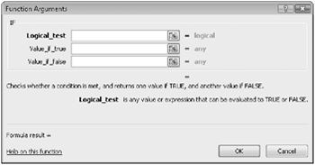
Another use for formulas is to display messages when certain conditions are met. For instance, Consolidated Messenger’s VP of Marketing, Craig Dewar, might have agreed to examine the rates charged to corporate customers who were billed for more than $100,000 during a calendar year. This kind of formula is called a conditional formula, and it uses the IF function. To create a conditional formula, you click the cell to hold the formula and open the Insert Function dialog box. From within the dialog box, select IF from the list of available functions and then click OK. The Function Arguments dialog box appears.

When you work with an IF function, the Function Arguments dialog box has three boxes: Logical_test, Value_if_true, and Value_if_false. The Logical_test box holds the condition you want to check. If the customer’s year-to-date shipping bill appears in cell G8, the expression would be G8>100000.

Now you need to have Excel 2007 display messages that indicate whether Craig Dewar should evaluate the account for a possible rate adjustment. To have Excel 2007 print a message from an IF function, you enclose the message in quotes in the Value_if_true or Value_if_false box. In this case, you would type “High-volume shipper-evaluate for rate decrease.” in the Value_if_true box and “Does not qualify at this time.” in the Value_if_false box.

Excel 2007 also includes five new conditional functions with which you can summarize your data:

• IFERROR, which displays one value if a formula results in an error; another if it doesn’t

• AVERAGEIF, which finds the average of values within a cell range that meet a given criterion

• AVERAGEIFS, which finds the average of values within a cell range that meet multiple criteria

• SUMIFS, which finds the sum of values in a range that meet multiple criteria

• COUNTIFS, which counts the number of cells in a range that meet multiple criteria

The IFERROR function enables you to display a custom error message instead of relying on the default Excel 2007 error messages to explain what happened. One example of an IFERROR formula is if you want to look up the CustomerID value from cell G8 in the Customers table by using the VLOOKUP function. One way to create such a formula is =IFERROR(VLOOKUP(G8,Customers,2,false),”Customer not found”). If the function finds a match for the CustomerID in cell G8, it displays the customer’s name; if it doesn’t find a match, it displays the text Customer not found.

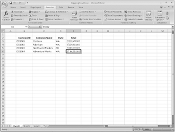
The AVERAGEIF function is a variation on the existing COUNTIF and SUMIF functions. To create a formula using the AVERAGEIF function, you define the range to be examined, the criteria, and, if required, the range from which to draw the values. As an example, consider the following worksheet, which lists each customer’s name, state, and total monthly shipping bill.

If you want to find the average order of customers from Washington State (abbreviated in the worksheet as WA), you can create the formula =AVERAGEIF(D3:D6,”=WA”, E3:E6).

The AVERAGEIFS, SUMIFS, and COUNTIFS functions extend the capabilities of the AVERAGEIF, SUMIF, and COUNTIF functions to allow for multiple criteria. If you want to find the sum of all orders of at least $100,000 placed by companies in Washington, you can create the formula =SUMIFS(E3:E6, D3:D6, “=WA”, E3:E6, “>=100000”).

The AVERAGEIFS and SUMIFS functions start with a data range that contains values that the formula summarizes; you then list the data ranges and the criteria to apply to that range. In generic terms, the syntax runs =AVERAGEIFS(data_range, criteria_range1,criteria1[,criteria_range2, criteria2…]). The part of the syntax in square brackets is optional, so an AVERAGEIFS or SUMIFS formula that contains a single criterion works. The COUNTIFS function, which doesn’t perform any calculations, doesn’t need a data range-you just provide the criteria ranges and criteria. For example, you could find the number of customers from Washington billed at least $100,000 by using the formula =COUNTIFS(D3:D6, “=WA”, E3:E6, “>=100000”).

In this exercise, you will create a conditional formula that displays a message if a condition is true, find the average of worksheet values that meet one criterion, and find the sum of worksheet values that meet two criteria.

Use the PackagingCosts workbook in the practice file folder for this topic. This practice file is located in the Formulas folder under SBS_Office2007.

Open the PackagingCosts workbook.

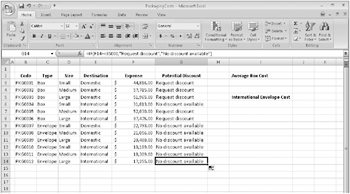
1. In cell G3, type the formula =IF(F3>=35000,”Request discount”,”No discount available”) and press .

Excel 2007 accepts the formula, which displays Request discount if the value in cell F3 is at least 35,000 and displays No discount available if not. The value Request discount appears in cell G3.

2. Click cell G3 and drag the fill handle down until it covers cell G14.

Excel 2007 copies the formula in cell G3 to cells G4:G14, adjusting the formula to reflect the cells’ addresses. The results of the copied formulas appear in cells G4:G14.

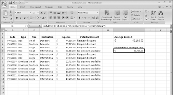
3. In cell I3, type the formula =AVERAGEIF(C3:C14, “=Box”, F3:F14) and press .

The value $46,102.50, which represents the average cost per category of boxes, appears in cell I3.

4. In cell I6, type =SUMIFS(F3:F14, C3:C14, “=Envelope”, E3:E14, “=International”).

The value $45,753.00, which represents the total cost of all envelopes used for international shipments, appears in cell I6.

Close the PackagingCosts workbook.