Applying Conditional Formatting

Formatting involves changing the size, font, color, bolding, underlining, and other characteristics of text. Conditional formatting involves changing text properties if specific conditions are met.

To understand conditional formatting, imagine an electronic digital kitchen timer. When the time reaches zero, usually an audible beep sounds, a bell rings, the number flashes, or something similar occurs. You can apply this same kind of behavior to the formats of one or more worksheet cells. If a cell value were less than the number 100, for instance, you could display the value in red. Similarly, if a cell value were greater than 1000, you could change the cell’s background color to green.

Applying conditional formatting is most helpful when you want to scan a list of values and note anomalies such as numbers that are above or below certain thresholds that can be harmful to your business. For example, if an insurance policy holder makes a claim for more than $5,000.00, you might want to display the claim amount in red.

In Excel, you can easily change the following cell properties:

• The font type

• Whether the font is bold, italic, or both

• The font’s size

• Whether the font has a single or double underline

• Whether the font has strikethrough, superscripted, or subscripted formatting

• The font color

• To which edges of a border special line thickness will be applied

• The border thickness

• The border color

• The cell’s background shading color

• The cell’s background pattern type, such as dashes, dots, or lines

To apply conditional formatting to one or more worksheet cells, select the cells to which you want to apply the formatting. Then, on the Format menu, click Conditional Formatting. Provide the conditional formatting properties in the Condition 1 area. If you want to add more cell formatting options, click the Add button and provide the conditional formatting properties in the Condition 2 area. (You can create up to three conditional formats per cell.) Finally, click the OK button to apply the conditional formatting.

Your Turn

In this exercise, you will color red all the cells in the Nights Booked column whose value is 5 or less, apply yellow to a cell if its value is 6 to 14, and apply green if the value is 15 or more.

1. Open Hotel.xls. If the file is already open, close it (do not save it) and open it again.

2. Select cells C2 through C313 in column C, the Nights Booked column.

3. On the Format menu, click Conditional Formatting.

4. In the Condition 1 area’s Between list, select Less Than Or Equal To.

5. In the box to the right, type 5.

6. Click Format, and then click the Patterns tab.

7. Click a red-colored box, and then click OK.

8. Click Add.

9. In the boxes next to the Condition 2 area’s Between list, type 6 in the first box and 14 in the second box.

10. Click Format, click a yellow-colored box on the Patterns tab, and then click OK.

11. Click Add. In the Condition 3 area’s Between list, select Greater Than Or Equal To, and then type 15 in the box to the right. Click Format, and then click a green-colored box on the Patterns tab.

12. Click OK, and compare your results to Figure 3-10.

    
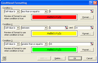
    Figure 3-10: The Conditional Formatting dialog box set up to highlight values in the number of nights booked.

13. Click OK, and compare your results to Figure 3-11.

    
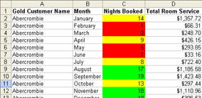
    Figure 3-11: Nights booked with conditional formatting.

Conditional formatting can really help you spot individual data values more quickly.