Exercises

• 5.1 Show that the two definitions of expectation for probability measures, (5.1) and (5.2), coincide if all sets are measurable.

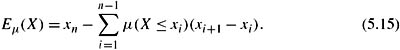
• 5.2 Prove (5.3) (under the assumption that X = x_i is measurable for i = 1, …, n).

• 5.3 Prove that

  

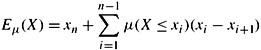
  and that

  

• 5.4 Prove Proposition 5.1.1.

• * 5.5 Show that E is (a) additive, (b) affinely homogeneous, and (c) monotone iff E is (a′) additive, (b′) positive (in the sense that if X ≥ 0 then E(x) ≥ 0), and Thus, in light of Proposition 5.1.1, (a′), (b′), and (c′) together give an alternate characterization of E_μ.

• * 5.6 Show that if μ is a countably additive probability measure, then (5.4) holds. Moreover, show that if E maps gambles that are measurable with respect to a σ-algebra to ℝ, and E is additive, affinely homogeneous, and monotone and satisfies (5.4), then E = E_μ for a unique countably additive probability measure μ on .

• * 5.7 Up to now I have focused on finite sets of worlds. This means that expectation can be expressed as a finite sum. With infinitely many worlds, new subtleties arise because infinite sums are involved. As long as the random variable is always positive, the problems are minor (although it is possible that the expected value of the variable may be infinite). If the random variable is negative on some worlds, then the expectation may not be well defined. This is a well-known problem when dealing with infinite sums, and has nothing to do with expectation per se. For example, consider the finite sum 1 − 1 + 1 − 1 + …. If this is grouped as (1 − 1) + (1 − 1) + …, then the sum is 0. However, if it is grouped as 1 − (1 − 1) − (1 − 1) + …, then the sum is 1. Having negative numbers in the sum does not always cause problems, but, when it does, the infinite sum is taken to be undefined.

  To see how this issue can affect expectation, consider the following two-envelope puzzle. Suppose that there are two envelopes, A and B. You are told that one envelope has twice as much money as the other and that you can keep whatever amount is in the envelope you choose. You choose envelope A. Before opening it, you are asked if you want to switch to envelope B and take the money in envelope B instead. You reason as follows. Suppose that envelope A has $n. Then with probability 1/2, envelope B has 2n, and with probability 1/2, envelope B has $n/2. Clearly you will gain $n if you stick with envelope A. If you choose envelope B, with probability 1/2, you will get $2n, and with probability 1/2, you will get $n/2. Thus, your expected gain is $(n + n/4), which is clearly greater than $n. Thus, it seems that if your goal is to maximize your expected gain, you should switch. But a symmetric argument shows that if you had originally chosen envelope B and were offered a chance to switch, then you should also do so.

  That seems very strange. No matter what envelope you choose, you want to switch! To make matters even worse, there is yet another argument showing that you should not switch. Suppose that envelope B has $n. Then, A has either $2n or $n/2, each with probability 1/2. With this representation, the expected gain of switching is $n and the expected gain of sticking with A is $5n/4.

  The two-envelope puzzle, while on the surface quite similar to the Monty Hall problem discussed in Chapter 1 (which will be analyzed formally in Chapter 6), is actually quite different. The first step in a more careful analysis is to construct a formal model. One thing that is missing in this story is the prior probability. For definiteness, suppose that there are infinitely many slips of paper, p₀, p₁, p₂, …. On slip p_i is written the pair of numbers (2ⁱ, 2ⁱ⁺¹) (so that p₀ has (1, 2), p₁ has (2, 4), etc.). Then p_i is chosen with probability α_i and the slip is cut in half; one number is put in envelope A, the other in envelope B, with equal probability. Clearly at this point—whatever the choice of α_i— the probabilities match those in the story. It really is true that one envelope has twice as much as the other. However, the earlier analysis does not apply. Suppose that you open envelope A and find a slip of paper saying $32. Certainly envelope B has either $16 or $64, but are both of these possibilities equally likely?

  1. Show that it is equally likely that envelope B has $16 or $64, given that envelope A has $32, if and only if α₄ = α₅.

  2. Similarly, show that, if envelope A contains 2^k for some k ≥ 1, then envelope is equally likely to contain 2^k−1 and 2^k+1 iff α_{k −1} = α_k. (Of course, if envelope A has $1, then envelope B must have $2.)

     It must be the case that ∑^∞_i=0 α_i = 1(since, with probability 1, some slip is chosen). It follows that the α_is cannot all be equal. Nevertheless, there is still a great deal of scope in choosing them. The problem becomes most interesting if α_i+1/α_i > 1/2. For definiteness, suppose that α_i = 1/3(2/3)ⁱ. This means α_i+1/α_i = 2/3.

  3. Show that ∑^∞_i=0 α_i = 1, so this is a legitimate choice of probabilities.

  4. Describe carefully a set of possible worlds and a probability measure μ on them that corresponds to this instance of the story.

  5. Show that, for this choice of probability measure μ, if k ≥ 2, then

     

  6. Show that, as a consequence, no matter what envelope A has, the expected gain of switching is greater than 0. (A similar argument shows that, no matter what envelope B has, the expected gain of switching is greater.)

     This seems paradoxical. If you choose envelope A, no matter what you see, you want to switch. This seems to suggest that, even without looking at the envelopes, if you choose envelope A, you want to have envelope B. Similarly, if you choose envelope B, you want to have envelope A. But that seems absurd. Clearly, your expected winnings with both A and B are the same. Indeed, suppose the game were played over and over again. Consider one person who always chose A and kept it, compared to another who always chose A and then switched to B. Shouldn't they expect to win the same amount? The next part of the exercise examines this a little more carefully.

  7. Suppose that you are given envelope A and have two choices. You can either keep envelope A (and get whatever amount is on the slip in envelope A) or switch to envelope B (and get whatever amount is on the slip in envelope B). Compute the expected winnings of each of the two choices. That is, if X_keep is the random variable that describes the amount you gain if you keep envelope A and X_switch is the random variable that describes the amount you win if you switch to envelope B, compute E_μ(X_keep) and E_μ(X_switch).

  8. What is E_μ(X_switch − X_keep)?

     If you did part (h) right, you should see that E_μ(X_switch − X_keep) is undefined. There are two ways of grouping the infinite sum that give different answers. In fact, one way gives an answer of 0 (corresponding to the intuition that it doesn't matter whether you keep A or switch to B; either way your expected winnings are the same) while another gives a positive answer (corresponding to the intuition that you're always better off switching). Part (g) helps explain the paradox. Your expected winnings are infinite either way (and, when dealing with infinite sums, ∞ + a = ∞ for any finite a).

• 5.8 Prove Proposition 5.2.1. Show that the restriction to positive affine homogeneity is necessary; in general, E_μ(aX) ≠ aE_μ(x) and E_μ(aX) ≠ aE_μ(x) if a < 0.

• * 5.9 Show that a function mapping gambles to ℝ is superadditive, positively affinely homogeneous, and monotone iff E is superadditive, E(cX) = cE(x), and E(x) ≥ inf{X(w) : w ∈ W}. In light of Theorem 5.2.2, the latter three properties provide an alternate characterization of ≤.

• 5.10 Show that if the smallest closed convex set of probability measures containing and ′ is the same, then E = E_′. (The notes to Chapters 2 and 3 have the definitions of convex and closed, respectively.) It follows, for example, that if W ={0, 1} and μ_α is the probability measure on W such that μ (0) = α, = {μ_α0, μ_α1}, and ′ = {μ_α : α₀ ≤ α ≤ α₁}, then ≤ = ≤′.

• 5.11 Some of the properties in Proposition 5.2.1 follow from others. Show in particular that all the properties of E given in parts (a)–(c) of Lemma 5.2.1 follow from the corresponding property of E and part (d) (i.e., the fact that E(X = − E(−X)). Moreover, show that it follows from these properties that

  

• 5.12 Show that (5.6), (5.7), and (5.8) hold if consists of countably additive measures.

• 5.13 Prove Proposition 5.2.3.

• 5.14 Prove Proposition 5.2.4.

• * 5.15 Prove Proposition 5.2.5.

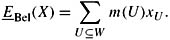
• * 5.16 Show that expectation for belief functions can be defined in terms of mass functions as follows. Given a belief function Bel with corresponding mass function m on a set W and a random variable X, let x_U = min_w∈U X(w). Show that

  

• 5.17 Show that

  

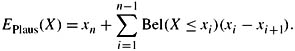
  Thus, the expression (5.15) for probabilistic expectation discussed in Exercise 5.3 can be used to define expectation for plausibility functions, using belief instead of probability. Since E_Bel(X) ≠ E_Plaus(X) in general, it follows that although (5.3) and (5.15) define equivalent expressions for probabilistic expectation, for other representations of uncertainty, they are not equivalent.

• * 5.18 Show that E_Bel satisfies (5.11). (Hint: Observe that if X and Y are random variables, then (X ∨ Y>x) = (X > x) ∪ (Y > x) and (X ∧ Y > x) = (X > x) ∩ (Y > x), and apply Proposition 5.2.5.)

• * 5.19 Show that E_Bel satisfies (5.12). (Hint: Observe that if X and Y are comonotonic, then it is possible to write X as a₁X_U1 + … + a_nX_Un and Y as b₁X_U1 + … + b_nX_Un, where the U_is are pairwise disjoint, a_i ≤ a_j iff i ≤ j, and b_i ≤ b_j iff i ≤ j. The result then follows easily from Proposition 5.2.5.)

• 5.20 Show that if X is a gamble such that (X) = {x₁,…, x_n} and x₁ < x₂ < … < x_n, and

  

  for j = 1, …, n, then (a) X = X_n and (b) X_j and (x_j+1 − x_j)X_X>xj are comonotonic, for j = 1, …, n − 1.

• 5.21 Prove Lemma 5.2.9. (Hint: First show that E(aX) = aE(x) for a a positive natural number, by induction, using the fact that E satisfies comonotonic additivity. Then show it for a a rational number. Finally, show it for a a real number, using the fact that E is monotone.)

• 5.22 Show E_Bel is the unique function E mapping gambles to ℝ that is superadditive, positively affinely homogeneous, and monotone and that satisfies (5.11) and (5.12) such that E(X_U) = Bel(U) for all U ⊆ W.

• 5.23 Show explicitly that, for the set of probability measures constructed in Example 5.2.10, _* is not a belief function.

• 5.24 Show that E′_μ(X) =−E′_μ(−X).

• * 5.25 Prove Lemma 5.2.13.

• 5.26 Prove Theorem 5.2.14. (You may assume Lemma 5.2.13.)

• 5.27 Prove Proposition 5.2.15.

• 5.28 Find gambles X and Y and a possibility measure Poss for which E_Poss(X ∨ Y) ≠ max(E_Poss(X), E_Poss(Y)).

• 5.29 Prove Proposition 5.2.16.

• 5.30 Let E′_Poss(X) = max_x∊(X) Poss(X = x)x. Show that E′_Poss satisfies monotonicity, the sup property, and the following three properties:

  

  

  

  Moreover, show that if E maps gambles to ℝ and satisfies monotonicity, the sup property, (5.16), (5.17), and (5.18), then there is a possibility measure Poss such that E = E′_Poss.

• 5.31 Let

  

  Show that for all b ≥ 1. This suggests that E″_Poss is not a reasonable definition of expectation for possibility measures.

• 5.32 Prove analogues of Propositions 5.1.1 and 5.1.2 for E_κ (replacing and + by + and min, respectively).

• 5.33 Verify that E_Pl,EDD = E_Pl.

• * 5.34 Show that . Then define natural sufficient conditions on ⊕, ⊗, and Pl that guarantee that E_Pl is (a) monotone, (b) superadditive, (c) additive, and (d) positively affinely homogeneous.

• 5.35 Given a utility function u on C and real numbers a > 0 and b, let the utility function u_a,b = au + b. That is, u_a,b(c) = au(c) + b for all c ∈ C. Show that the order on acts is the same for u and u_a,b according to (a) the expected utility maximization rule, (b) the maximin rule, and (c) the minimax regret rule. This result shows that these three decision rules are unaffected by positive affine transformations of the utilities.

• 5.36 Show that if _W is the set of all probability measures on W, then E_W(u_a) = worst_u. Thus, a ≽ a′ iff worst_u(a) ≥ worst_u(a′).

• 5.37 Show that if aa′ then a.

• 5.38 Prove Theorem 5.4.2. (Hint: Given DS = (A, W, C), let the expectation domain ED = (D₁, D₂, D₃, ⊕, ⊗) be defined as follows:

  • D₁ = 2^W, partially ordered by ⊆.

  • D₂ = C, and c₁ ≤₂ c₂ if a_c1 ≼_A a_c2, where a_ci is the constant act that returns c_i in all worlds in W.

  • D₃ consist of all subsets of W C. (Note that since a function can be identified with a set of ordered pairs, acts in A can be viewed as elements of D₃.)

  • x⊕ y = x ∪ y for x, y ∈ D₃; for U ∈D₁ and c ∈D₂, define U ⊗ c = U {c}.

  • The preorder ≤₃ on D₃ is defined by taking x ≤ y iff x = y or x = a and y = a′ for some acts a, a′ ∈ A such that a ≼_A a′.

  Note that D₂ can be viewed as a subset of D₃ by identifying c ∈ D₂ with W {c}. With this identification, ≤₂ is easily seen to be the restriction of ≤₃ to D₂. Define Pl(U) = U for all U ⊆ W. Show that E_{Pl, ED}(u_a) = a.)

• 5.39 Fill in the details showing that GEU can represent maximin. In particular, show that E_{Plmax, EDmax}(u_a) = worst_u(a) for all actions a ∈ A.

• 5.40 This exercise shows that GEU can represent a generalized version of maximin, where the range of the utility function is an arbitrary totally ordered set. If DP = (DS, D, u), where D is totally preordered by ≤_D, then let τ(DP) = (DS, ED_{max, D}, Pl_{max, D}, u), where ED_{max, D} = ({0, 1}, D, D, min, ⊗), 0 ⊗ x = 1 ⊗ x = x for all x ∈ D, and Pl_{max, D} is defined as in the real-valued case; that is, Pl_{max, D}(U) is 1 if U ≠ ∅ and 0 if U =∅. Show that ED_{max, D} is an expectation domain and that GEU(τ(DP)) = maximin(DP).

• 5.41 Show that if M_DP = ∞, then all acts have infinite regret.

• 5.42 Show that E_{PlDP, EDreg}(u_a) = M_DP − regret_u(a) for all acts a ∈ A.

• * 5.43 Prove Theorem 5.4.4. (Hint: Use a construction much like that used in Exercise 5.38 to prove Theorem 5.4.2.)

• 5.44 Show that if Pl_Bel(U) ≤ Pl_Bel(V) then Bel(U) ≤ Bel(V), but the converse does not hold in general.

• * 5.45 This exercise shows that GEU ordinally represents 퓓_BEL.

  1. Define a partial preorder ≤ on D 2^W by taking (f, U) ≤ (g, V) iff inf_i∈I f(i) ≤ inf_i∈I g(i). Show that ≤ is a partial preorder, although not a partial order.

  2. Given a belief function Bel, define Pl′_Bel by taking Pl′_Bel(U) = Pl_Bel (U), U). Show that Pl′_Bel is a plausibility measure that represents the same ordinal tastes as Bel. (Note that for the purposes of this exercise, the range of a plausibility measure can be partially preordered.)

  3. Define an expectation domain ED′_D such that

     

• * 5.46 Prove Theorem 5.4.6. (Hint: Combine ideas from Exercises 5.38 and 5.45.)

• 5.47 Show that E_μ(X_V | U) = μ(V | U).

• 5.48 Show that E_Bel(X | U) = E_{Bel |U} (X).

• 5.49 Show that conditional expectation can be used as a tool to calculate unconditional expectation. More precisely, show that if V₁, …, V_n is a partition of W and X is a random variable over W, then

  

  (Compare this result with Lemma 3.9.5.)

• 5.50 Prove Lemma 5.5.1.

• 5.51 Prove Lemma 5.5.2.