2.4 Dempster-Shafer Belief Functions

2.4 Dempster-Shafer Belief Functions

The Dempster-Shafer theory of evidence, originally introduced by Arthur Dempster and then developed by Glenn Shafer, provides another approach to attaching likelihood to events. This approach starts out with a belief function (sometimes called a support function). Given a set W of possible worlds and U ⊆ W, the belief in U, denoted Bel(U), is a number in the interval [0, 1]. (Think of Bel as being defined on the algebra 2^W consisting of all subsets of W. The definition can easily be generalized so that the domain of Bel is an arbitrary algebra over W, although this is typically not done in the literature.) A belief function Bel defined on a space W must satisfy the following three properties:

• B1. Bel(⊘) = 0.

• B2. Bel(W) = 1.

• B3. Bel(∪ⁿ_{i = 1} U_i) ≥ Σⁿ_{i = 1} Σ_{{I⊆{1, …, n}:|I|=i}}(−1)^{I + 1} Bel (∩_{j ∈ I} U_j), for n = 1, 2, 3, ….

If W is infinite, Bel is sometimes assumed to satisfy the continuity property that results by replacing μ in (2.2) by Bel:

The reason that the analogue of (2.2) is considered rather than (2.1) should shortly become clear. In any case, like countable additivity, this is a property that is not always required.

B1 and B2 just say that, like probability measures, belief functions follow the convention of using 0 and 1 to denote the minimum and maximum likelihood. B3 is just the inclusion-exclusion rule with = replaced by ≥. Thus, every probability measure defined on 2^W is a belief function. Moreover, from the results of the previous section, it follows that every inner measure is a belief function as well. The converse does not hold; that is, not every belief function is an inner measure corresponding to some probability measure. For example, if W ={w, w′}, Bel(w) = 1/2, Bel(w′) = 0, Bel(W) = 1, and Bel(∅) = 0, then Bel is a belief function, but there is no probability measure μ on W such that Bel = μ_* (Exercise 2.20). On the other hand, Exercise 7.11 shows that there is a sense in which every belief function can be identified with the inner measure corresponding to some probability measure.

A probability measure defined on 2^W can be characterized by its behavior on singleton sets. This is not the case for belief functions. For example, it is easy to construct two belief functions Bel₁ and Bel₂ on {1, 2, 3} such that Bel₁(i) = Bel₂(i) = 0 for i = 1, 2, 3 (so that Bel₁ and Bel₂ agree on singleton sets) but Bel₁({1, 2}) ≠ Bel₂({1, 2}) (Exercise 2.21). Thus, a belief function cannot be viewed as a function on W ; its domain must be viewed as being 2^W (or some algebra over W ). (The same is also true for 풫^* and 풫_*. It is easy to see this directly; it also follows from Theorem 2.4.1, which says that every belief function is 풫_* for some set 풫 of probability measures.)

Just like an inner measure, Bel(U) can be viewed as providing a lower bound on the likelihood of U. Define Plaus(U) = 1 − Bel(U). Plaus is a plausibility function; Plaus(U) is the plausibility of U. A plausibility function bears the same relationship to a belief function that an outer measure bears to an inner measure. Indeed, every outer measure is a plausibility function. It follows easily from B3 (applied to U and U, with n = 2) that Bel(U) ≤ Plaus(U) (Exercise 2.22). For an event U, the interval [Bel(U), Plaus(U)] can be viewed as describing the range of possible values of the likelihood of U. Moreover, plausibility functions satisfy the analogue of (2.9):

(Exercise 2.13). Indeed, plausibility measures are characterized by the properties Plaus(∅) = 0, Plaus(W) = 1, and (2.16).

These observations show that there is a close relationship among belief functions, inner measures, and lower probabilities. Part of this relationship is made precise by the following theorem:

Theorem 2.4.1

Given a belief function Bel defined on a space W, let 풫_Bel = {μ : μ (U) ≥ Bel(U) for all U ⊆ W. Then Bel = (풫_Bel)_* and Plaus = (풫_Bel)^*.

Proof See Exercise 2.23.

Theorem 2.4.1 shows that every belief function on W can be viewed as a lower probability of a set of probability measures on W. That is why (2.15) seems to be the appropriate continuity property for belief functions, rather than the analogue of (2.1).

The converse of Theorem 2.4.1 does not hold. It follows from Exercise 2.14 that lower probabilities do not necessarily satisfy the analogue of (2.8), and thus there is a space W and a set 풫 of probability measures on W such that no belief function Bel on W with Bel = 풫_* exists. For future reference, it is also worth noting that, in general, there may be sets 풫 other than 풫_Bel such that Bel = 풫_* and Plaus = 풫^* (Exercise 2.24).

In any case, while belief functions can be understood (to some extent) in terms of lower probability, this is not the only way of understanding them. Belief functions are part of a theory of evidence. Intuitively, evidence supports events to varying degrees. For example, in the case of the marbles, the information that there are exactly 30 red marbles provides support in degree .3 for red; the information that there are 70 yellow and blue marbles does not provide any positive support for either blue or yellow, but does provide support .7 for {blue, yellow}. In general, evidence provides some degree of support (possibly 0) for each subset of W. The total amount of support is 1. The belief that U holds, Bel(U), is then the sum of all of the support on subsets of U.

Formally, this is captured as follows. A mass function (sometimes called a basic probability assignment)on W is a function m :2^W → [0, 1] satisfying the following properties:

• M1. m (⊘) = 0.

• M2. Σ_{U ⊆ W} ^{m(U) = 1.}

Intuitively, m(U) describes the extent to which the evidence supports U. This is perhaps best understood in terms of making observations. Suppose that an observation U is accurate, in that if U is observed, the actual world is in U. Then m(U) can be viewed as the probability of observing U. Clearly it is impossible to observe ∅ (since the actual world cannot be in ∅), so m(∅) = 0. Thus, M1 holds. On the other hand, since something must be observed, M2 must hold.

Given a mass function m, define the belief function based on m, Bel_m, by taking

Intuitively, Bel_m(U) is the sum of the probabilities of the evidence or observations that guarantee that the actual world is in U. The corresponding plausibility function Plaus_m is defined as

(If U =∅, the sum on the right-hand side of the equality has no terms; by convention, it is taken to be 0.) Plaus_m(U) can be thought of as the sum of the probabilities of the evidence that is compatible with the actual world being in U.

Example 2.4.2

Suppose that W ={w₁, w₂, w₃}. Define m as follows:

• m(w₁) = 1/4;

• m({w₁, w₂}) = 1/4;

• m({w₂, w₃}) = 1/2;

• m(U) = 0 if U is not one of {w₁}, {w₁, w₂}, or {w₁, w₃}.

Then it is easy to check that

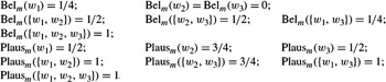
Although I have called Bel_m a belief function, it is not so clear that it is. While it is obvious that Bel_m satisfies B1 and B2, it must be checked that it satisfies B3. The following theorem confirms that Bel_m is indeed a belief function. It shows much more though: it shows that every belief function is Bel_m for some mass function m. Thus, there is a one-to-one correspondence between belief functions and mass functions.

Theorem 2.4.3

Given a mass function m on a finite set W, the function Bel_m is a belief function and Plaus_m is the corresponding plausibility function. Moreover, given a belief function Bel on W, there is a unique mass function m on W such that Bel = Bel_m.

Proof See Exercise 2.25.

Bel_m and its corresponding plausibility function Plaus_m are the belief function and plausibility function corresponding to the mass function m.

Theorem 2.4.3 is one of the few results in this book that depends on the set W being finite. While it is still true that to every mass function there corresponds a belief function even if W is infinite, there are belief functions in the infinite case that have no corresponding mass functions (Exercise 2.26).

Since a probability measure μ on 2^W is a belief function, it too can be characterized in terms of a mass function. It is not hard to show that if μ is a probability measure on 2^W, so that every set is measurable, the mass function m_μ corresponding to μ gives positive mass only to singletons and, in fact, m_μ(w) = μ(w) for all w ∈ W. Conversely, if m is a mass function that gives positive mass only to singletons, then the belief function corresponding to m is in fact a probability measure on (Exercise 2.27).

Example 2.3.2 can be captured using the function m such that m(red) = .3, m(blue) = m(yellow) = m({red, blue, yellow}) = 0, and m({blue, yellow}) = .7. In this case, m looks like a probability measure, since the sets that get positive mass are disjoint, and the masses sum to 1. However, in general, the sets of positive mass may not be disjoint. It is perhaps best to think of m(U) as the amount of belief committed to U that has not already been committed to its subsets. The following example should help make this clear:

Example 2.4.4

Suppose that a physician sees a case of jaundice. He considers four possible hypotheses regarding its cause: hepatitis (hep), cirrhosis (cirr), gallstone (gall), and pancreatic cancer (pan). For simplicity, suppose that these are the only causes of jaundice, and that a patient with jaundice suffers from exactly one of these problems. Thus, the physician can take the set W of possible worlds to be {hep, cirr, gall, pan}. Only some subsets of 2^W are of diagnostic significance. There are tests whose outcomes support each of the individual hypotheses, and tests that support intrahepatic cholestasis, {hep, cirr}, and extrahepatic cholestasis, {gall, pan}; the latter two tests do not provide further support for the individual hypotheses.

If there is no information supporting any of the hypotheses, this would be represented by a mass function that assigns mass 1 to W and mass 0 to all other subsets of W. On the other hand, suppose there is evidence that supports intrahepatic cholestasis to degree .7. (The degree to which evidence supports a subset of W can be given both a relative frequency and a subjective interpretation. Under the relative frequency interpretation, it could be the case that 70 percent of the time that the test had this outcome, a patient had hepatitis or cirrhosis.) This can be represented by a mass function that assigns .7 to {hep, cirr} and the remaining .3 to W. The fact that the test provides support only .7 to {hep, cirr} does not mean that it provides support .3 for its complement, {gall, pan}. Rather, the remaining .3 is viewed as uncommitted. As a result, Bel({hep, cirr}) = .7 and Plaus({hep, cirr}) = 1.

Suppose that a doctor performs two tests on a patient, each of which provides some degree of support for a particular hypothesis. Clearly the doctor would like some way of combining the evidence given by these two tests; the Dempster-Shafer theory provides one way of doing this.

Let Bel₁ and Bel₂ denote two belief functions on some set W, and let m₁ and m₂ be their respective mass functions. Dempster's Rule of Combination provides a way of constructing a new mass function m₁ ⊕ m₂, provided that there are at least two sets U₁ and U₂ such that U₁ ∩ U₂ ≠∅ and m₁(U₁)m₂(U₂)> 0. If there are no such sets U₁ and U₂, then m₁ ⊕ m₂ is undefined. Notice that, in this case, there must be disjoint sets V₁ and V₂ such that Bel₁(V₁) = Bel₂(V₂) = 1 (Exercise 2.28). Thus, Bel₁ and Bel₂ describe diametrically opposed beliefs, so it should come as no surprise that they cannot be combined.

The intuition behind the Rule of Combination is not that hard to explain. Suppose that an agent obtains evidence from two sources, one characterized by m₁ and the other by m₂. An observation U₁ from the first source and an observation U₂ from the second source can be viewed as together providing evidence for U₁ ∩ U₂. Roughly speaking then, the evidence for a set U₃ should consist of the all the ways of observing sets U₁ from the first source and U₂ from the second source such that U₁ ∩ U₂ = U₃. If the two sources are independent (a notion discussed in greater detail in Chapter 4), then the likelihood of observing both U₁ and U₂ is the product of the likelihood of observing each one, namely, m₁(U₁)m₂(U₂). This suggests that the mass of U₃ according to m₁ ⊕ m₂ should be ∑_{{U1, U2:U1∩U2=U3}} m₁(U₁)m₂(U₂). This is almost the case. The problem is that it is possible that U₁ ∩ U₂ =∅. This counts as support for the true world being in the empty set, which is, of course, impossible. Such a pair of observations should be ignored. Thus, m₃(U) is the sum of m₁(U₁)m₂(U₂) for all pairs (U₁, U₂) such that U₁ ∩ U₂ ≠∅, conditioned on not observing pairs whose intersection is empty. (Conditioning is discussed in Chapter 3. I assume here that the reader has a basic understanding of how conditioning works, although it is not critical for understanding the Rule of Combination.)

Formally, define (m₁ ⊕ m₂)(∅) = 0 and for U ≠∅, define

where c = ∑_{{U1, U2:U1∩U2≠∅}} m₁(U₁)m₂(U₂). Note that c is can be thought of as the probability of observing a pair (U₁, U₂) such that U₁ ∩ U₂ ≠∅.If m₁ ⊕ m₂ is defined, then c > 0, since there are sets U₁, U₂ such that U₁ ∩ U₂ ≠∅ and m₁(U₁)m₂(U₂) > 0. Conversely, if c > 0, then it is almost immediate that m₁ ⊕ m₂ is defined and is a mass function (Exercise 2.29). Let Bel₁ ⊕ Bel₂ be the belief function corresponding to m₁ ⊕ m₂.

It is perhaps easiest to understand how Bel₁ ⊕ Bel₂ works in the case that Bel₁ and Bel₂ are actually probability measures μ₁ and μ₂, and all sets are measurable. In that case, Bel₁ ⊕ Bel₂ is a probability measure, where the probability of a world w is the product of its probability according to Bel₁ and Bel₂, appropriately normalized so that the sum is 1. To see this, recall that the corresponding mass functions m₁ and m₂ assign positive mass only to singleton sets and m_i(w) = μ_i(w) for i = 1, 2. Since m_i(U) = 0 if U is not a singleton for i = 1, 2, it follows easily that (m₁ ⊕ m₂)(U) = 0 if U is not a singleton, and (m₁ ⊕ m₂)(w) = μ₁(w)μ₂(w)/c, where c = ∑_w∈W μ₁(w)μ₂(w). Since m₁ ⊕ m₂ assigns positive mass only to singletons, the belief function corresponding to m₁ ⊕ m₂ is a probability measure. Moreover, it is immediate that (μ₁ ⊕ μ₂)(U) = ∑_{w ∈ U} μ₁(w)μ₂(w)/c.

It has been argued that the Dempster rule of combination is appropriate when combining two independent pieces of evidence. Independence is viewed as an intuitive, primitive notion here. Essentially, it says the sources of the evidence are unrelated. (See Section 4.1 for more discussion of this issue.) The rule has the attractive feature of being commutative and associative:

This seems reasonable. Final beliefs should be independent of the order and the way in which the evidence is combined. Let m_vac be the vacuous mass function on W : m_vac(W) = 1 and m(U) = 0 for U ⊂ W. It is easy to check that m_vac is the neutral element in the space of mass functions on W ; that is, m_vac ⊕ m = m ⊕ m_vac = m for every mass function m (Exercise 2.30).

Rather than going through a formal derivation of the Rule of Combination, I consider two examples of its use here, where it gives intuitively reasonable results. In Section 3.2, I relate it to the probabilistic combination of evidence.

Example 2.4.5

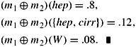
Returning to the medical situation in Example 2.4.4, suppose that two tests are carried out. The first confirms hepatitis to degree .8 and says nothing about the other hypotheses; this is captured by the mass function m₁ such that m₁(hep) = .8 and m₁(W) = .2. The second test confirms intrahepatic cholestasis to degree .6; it is captured by the mass function m₂ such that m₂({hep, cirr}) = .6 and m₂(W) = .4. A straightforward computation shows that

Example 2.4.6

Suppose that Alice has a coin and she knows that it either has bias 2/3(BH) or bias 1/3(BT). Initially, she has no evidence for BH or BT. This is captured by the vacuous belief function Bel_init, where Bel_init(BH) = Bel_init(BT) = 0 and Bel_init(W) = 1. Suppose that Alice then tosses the coin and observes that it lands heads. This should give her some positive evidence for BH but no evidence for BT. One way to capture this evidence is by using the belief function Bel_heads such that Bel_heads(BH) = α > 0 and Bel_heads(BT) = 0. (The exact choice of α does not matter.) The corresponding mass function m_heads is such that m_heads(BT) = 0, m_heads(BH) = α, and m_heads(W) = 1 − α. Mass and belief functions m_tails and Bel_tails that capture the evidence of tossing the coin and seeing tails can be similarly defined. Note that m_init ⊕ m_heads = m_heads, and similarly for m_tails. Combining Alice's initial ignorance regarding BH and BT with the evidence results in the same beliefs as those produced by just the evidence itself.

Now what happens if Alice observes k heads in a row? Intuitively, this should increase her degree of belief that the coin is biased toward heads. Let m^k_heads = m_heads ⊕ … ⊕ m_heads (k times). A straightforward computation shows that m^k_heads(BT) = 0, m^k_heads(BH) = 1 − (1 − α)^k, and m^k_heads(W) = (1 − α)^k. Observing heads more and more often drives Alice's belief that the coin is biased toward heads to 1.

Another straightforward computation shows that

Thus, as would be expected, after seeing heads and then tails (or, since ⊕ is commutative, after seeing tails and then heads), Alice assigns an equal degree of belief to BH and BT. However, unlike the initial situation where Alice assigned no belief to either BH or BT, she now assigns positive belief to each of them, since she has seen some evidence in favor of each.