Oracle is designed to be a very portable database - it is available on every platform of relevance. For this reason, the physical architecture of Oracle looks different on different operating systems. For example, on a UNIX operating system, you will see Oracle implemented as many different operating system processes, virtually a process per major function. On UNIX, this is the correct implementation, as it works on a multi-process foundation. On Windows however, this architecture would be inappropriate and would not work very well (it would be slow and non-scaleable). On this platform, Oracle is implemented as a single, threaded process, which is the appropriate implementation mechanism on this platform. On IBM mainframe systems running OS/390 and zOS, the Oracle operating system-specific architecture exploits multiple OS/390 address spaces, all operating as a single Oracle instance. Up to 255 address spaces can be configured for a single database instance. Moreover, Oracle works together with OS/390 WorkLoad Manager (WLM) to establish execution priority of specific Oracle workloads relative to each other, and relative to all other work in the OS/390 system. On Netware we are back to a threaded model again. Even though the physical mechanisms used to implement Oracle from platform to platform vary, the architecture is sufficiently generalized enough that you can get a good understanding of how Oracle works on all platforms.
In this chapter, we will look at the three major components of the Oracle architecture:
Files - we will go through the set of five files that make up the database and the instance. These are the parameter, data, temp, and redolog Files.
Memory structures, referred to as the System Global Area (SGA) - we will go through the relationships between the SGA, PGA, and UGA. Here we also go through the Java pool, shared pool, and large pool parts of the SGA.
Physical processes or threads - we will go through the three different types of processes that will be running on the database: server processes, background processes, and slave processes.
The Server
It is hard to decide which of these components to cover first. The processes use the SGA, so discussing the SGA before the processes might not make sense. On the other hand, by discussing the processes and what they do, I'll be making references to the SGA. The two are very tied together. The files are acted on by the processes and would not make sense without understanding what the processes do. What I will do is define some terms and give a general overview of what Oracle looks like (if you were to draw it on a whiteboard) and then we'll get into some of the details.
There are two terms that, when used in an Oracle context, seem to cause a great deal of confusion. These terms are 'instance' and 'database'. In Oracle terminology, the definitions would be:
Database - A collection of physical operating system files
Instance - A set of Oracle processes and an SGA
The two are sometimes used interchangeably, but they embrace very different concepts. The relationship between the two is that a database may be mounted and opened by many instances. An instance may mount and open a single database at any point in time. The database that an instance opens and mounts does not have to be the same every time it is started.
Confused even more? Here are some examples that should help clear it up. An instance is simply a set of operating system processes and some memory. They can operate on a database, a database just being a collection of files (data files, temporary files, redo log files, control files). At any time, an instance will have only one set of files associated with it. In most cases, the opposite is true as well; a database will have only one instance working on it. In the special case of Oracle Parallel Server (OPS), an option of Oracle that allows it to function on many computers in a clustered environment, we may have many instances simultaneously mounting and opening this one database. This gives us access to this single database from many different computers at the same time. Oracle Parallel Server provides for extremely highly available systems and, when implemented correctly, extremely scalable solutions. In general, OPS will be considered out of scope for this book, as it would take an entire book to describe how to implement it.
So, in most cases, there is a one-to-one relationship between an instance and a database. This is how the confusion surrounding the terms probably arises. In most peoples' experience, a database is an instance, and an instance is a database.
In many test environments, however, this is not the case. On my disk, I might have, five separate databases. On the test machine, I have Oracle installed once. At any point in time there is only one instance running, but the database it is accessing may be different from day to day or hour to hour, depending on my needs. By simply having many different configuration files, I can mount and open any one of these databases. Here, I have one 'instance' but many databases, only one of which is accessible at any point in time.
So now when someone talks of the instance, you know they mean the processes and memory of Oracle. When they mention the database, they are talking of the physical files that hold the data. A database may be accessible from many instances, but an instance will provide access to exactly one database at a time.
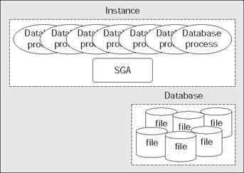
Now we might be ready for an abstract picture of what Oracle looks like:
In its simplest form, this is it. Oracle has a large chunk of memory call the SGA where it will: store many internal data structures that all processes need access to; cache data from disk; cache redo data before writing it to disk; hold parsed SQL plans, and so on. Oracle has a set of processes that are 'attached' to this SGA and the mechanism by which they attach differs by operating system. In a UNIX environment, they will physically attach to a large shared memory segment - a chunk of memory allocated in the OS that may be accessed by many processes concurrently. Under Windows, they simply use the C call malloc() to allocate the memory, since they are really threads in one big process. Oracle will also have a set of files that the database processes/threads read and write (and Oracle processes are the only ones allowed to read or write these files). These files will hold all of our table data, indexes, temporary space, redo logs, and so on.
If you were to start up Oracle on a UNIX-based system and execute a ps (process status) command, you would see that many physical processes are running, with various names. For example:
$ /bin/ps -aef | grep ora816 ora816 20827 1 0 Feb 09 ? 0:00 ora_d000_ora816dev ora816 20821 1 0 Feb 09 ? 0:06 ora_smon_ora816dev ora816 20817 1 0 Feb 09 ? 0:57 ora_lgwr_ora816dev ora816 20813 1 0 Feb 09 ? 0:00 ora_pmon_ora816dev ora816 20819 1 0 Feb 09 ? 0:45 ora_ckpt_ora816dev ora816 20815 1 0 Feb 09 ? 0:27 ora_dbw0_ora816dev ora816 20825 1 0 Feb 09 ? 0:00 ora_s000_ora816dev ora816 20823 1 0 Feb 09 ? 0:00 ora_reco_ora816dev
I will cover what each of these processes are, but they are commonly referred to as the Oracle background processes. They are persistent processes that make up the instance and you will see them from the time you start the database, until the time you shut it down. It is interesting to note that these are processes, not programs. There is only one Oracle program on UNIX; it has many personalities. The same 'program' that was run to get ora_lgwr_ora816dev, was used to get the process ora_ckpt_ora816dev. There is only one binary, named simply oracle. It is just executed many times with different names. On Windows, using the tlist tool from the Windows resource toolkit, I will find only one process, Oracle.exe. Again, on NT there is only one binary program. Within this process, we'll find many threads representing the Oracle background processes. Using tlist (or any of a number of tools) we can see these threads:
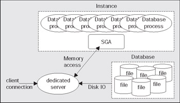
Here, there are eleven threads executing inside the single process Oracle. If I were to log into this database, I would see the thread count jump to twelve. On UNIX, I would probably see another process get added to the list of oracle processes running. This brings us to the next iteration of the diagram. The previous diagram gave a conceptual depiction of what Oracle would look like immediately after starting. Now, if we were to connect to Oracle in its most commonly used configuration, we would see something like:
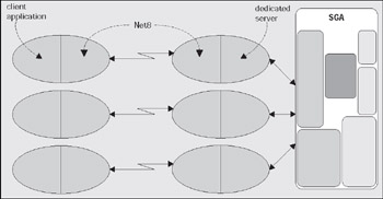
Typically, Oracle will create a new process for me when I log in. This is commonly referred to as the dedicated server configuration, since a server process will be dedicated to me for the life of my session. For each session, a new dedicated server will appear in a one-to-one mapping. My client process (whatever program is trying to connect to the database) will be in direct contact with this dedicated server over some networking conduit, such as a TCP/IP socket. It is this server that will receive my SQL and execute it for me. It will read data files, it will look in the database's cache for my data. It will perform my update statements. It will run my PL/SQL code. Its only goal is to respond to the SQL calls that I submit to it.
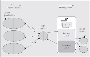
Oracle may also be executing in a mode called multi-threaded server (MTS) in which we would not see an additional thread created, or a new UNIX process appear. In MTS mode, Oracle uses a pool of 'shared servers' for a large community of users. Shared servers are simply a connection pooling mechanism. Instead of having 10000 dedicated servers (that's a lot of processes or threads) for 10000 database sessions, MTS would allow me to have a small percentage of this number of shared servers, which would be (as their name implies) shared by all sessions. This allows Oracle to connect many more users to the database than would otherwise be possible. Our machine might crumble under the load of managing 10000 processes, but managing 100 or 1000 processes would be doable. In MTS mode, the shared server processes are generally started up with the database, and would just appear in the ps list (in fact in my previous ps list, the process ora_s000_ora816dev is a shared server process).
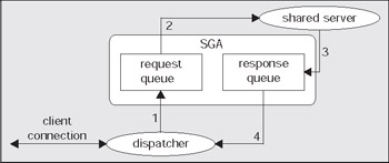
A big difference between MTS mode and dedicated server mode is that the client process connected to the database never talks directly to a shared server, as it would to a dedicated server. It cannot talk to a shared server since that process is in fact shared. In order to share these processes we need another mechanism through which to 'talk'. Oracle employs a process (or set of processes) called dispatchers for this purpose. The client process will talk to a dispatcher process over the network. The dispatcher process will put the client's request into a request queue in the SGA (one of the many things the SGA is used for). The first shared server that is not busy will pick up this request, and process it (for example, the request could be UPDATETSETX=X+5WHEREY=2. Upon completion of this command, the shared server will place the response in a response queue. The dispatcher process is monitoring this queue and upon seeing a result, will transmit it to the client. Conceptually, the flow of an MTS request looks like this:
The client connection will send a request to the dispatcher. The dispatcher will first place this request onto the request queue in the SGA (1). The first available shared server will dequeue this request (2) and process it. When the shared server completes, the response (return codes, data, and so on) is placed into the response queue (3) and subsequently picked up by the dispatcher (4), and transmitted back to the client.
As far as the developer is concerned, there is no difference between a MTS connection and a dedicated server connection. So, now that we understand what dedicated server and shared server connections are, this begs the questions, 'How do we get connected in the first place?' and 'What is it that would start this dedicated server?' and 'How might we get in touch with a dispatcher?' The answers depend on our specific platform, but in general, it happens as described below.
We will investigate the most common case - a network based connection request over a TCP/IP connection. In this case, the client is situated on one machine, and the server resides on another machine, the two being connected on a TCP/IP network. It all starts with the client. It makes a request to the Oracle client software to connect to database. For example, you issue:
C:\> sqlplus scott/tiger@ora816.us.oracle.com
Here the client is the program SQL*PLUS, scott/tiger is my username and password, and ora816.us.oracle.com is a TNS service name. TNS stands for Transparent Network Substrate and is 'foundation' software built into the Oracle client that handles our remote connections - allowing for peer-to-peer communication. The TNS connection string tells the Oracle software how to connect to the remote database. Generally, the client software running on your machine will read a file called TNSNAMES.ORA. This is a plain text configuration file commonly found in the [ORACLE_HOME]\network\admin directory that will have entries that look like:
It is this configuration information that allows the Oracle client software to turn ora816.us.oracle.com into something useful - a hostname, a port on that host that a 'listener' process will accept connections on, the SID (Site IDentifier) of the database on the host to which we wish to connect, and so on. There are other ways that this string, ora816.us.oracle.com, could have been resolved. For example it could have been resolved using Oracle Names, which is a distributed name server for the database, similar in purpose to DNS for hostname resolution. However, use of the TNSNAMES.ORA is common in most small to medium installations where the number of copies of such a configuration file is manageable.
Now that the client software knows where to connect to, it will open a TCP/IP socket connection to the machine aria.us.oracle.com on the port 1521. If the DBA for our server has setup Net8, and has the listener running, this connection may be accepted. In a network environment, we will be running a process called the TNS Listener on our server. This listener process is what will get us physically connected to our database. When it receives the inbound connection request, it inspects the request and, using its own configuration files, either rejects the request (no such database for example, or perhaps our IP address has been disallowed connections to this host) or accepts it and goes about getting us connected.
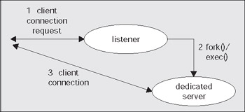
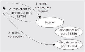
If we are making a dedicated server connection, the listener process will create a dedicated server for us. On UNIX, this is achieved via a fork() and exec() system call (the only way to create a new process after initialization in UNIX is fork()). We are now physically connected to the database. On Windows, the listener process requests the database process to create a new thread for a connection. Once this thread is created, the client is 'redirected' to it, and we are physically connected. Diagrammatically in UNIX, it would look like this:
On the other hand, if we are making a MTS connection request, the listener will behave differently. This listener process knows the dispatcher(s) we have running on the database. As connection requests are received, the listener will choose a dispatcher process from the pool of available dispatchers. The listener will send back to the client the connection information describing how the client can connect to the dispatcher process. This must be done because the listener is running on a well-known hostname and port on that host, but the dispatchers will be accepting connections on 'randomly assigned' ports on that server. The listener is aware of these random port assignments and picks a dispatcher for us. The client then disconnects from the listener and connects directly to the dispatcher. We now have a physical connection to the database. Graphically this would look like this:
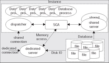
So, that is an overview of the Oracle architecture. Here, we have looked at what an Oracle instance is, what a database is, and how you can get connected to the database either through a dedicated server, or a shared server. The following diagram sums up what we've seen so far; showing the interaction between the a client using a shared server (MTS) connection and a client using a dedicated server connection. It also shows that an Oracle instance may use both connection types simultaneously:
Now we are ready to take a more in-depth look at the processes behind the server, what they do, and how they interact with each other. We are also ready to look inside the SGA to see what is in there, and what its purpose it. We will start by looking at the types of files Oracle uses to manage the data and the role of each file type.
The Files
We will start with the five types of file that make up a database and instance. The files associated with an instance are simply:
Parameter files - These files tell the Oracle instance where to find the control files. For example, how big certain memory structures are, and so on.
The files that make up the database are:
Data files - For the database (these hold your tables, indexes and all other segments).
Redo log files - Our transaction logs.
Control files - Which tell us where these data files are, and other relevant information about their state.
Temp files - Used for disk-based sorts and temporary storage.
Password files - Used to authenticate users performing administrative activities over the network. We will not discuss these files in any detail.
The most important files are the first two, because they contain the data you worked so hard to accumulate. I can lose any and all of the remaining files and still get to my data. If I lose my redo log files, I may start to lose some data. If I lose my data files and all of their backups, I've definitely lost that data forever.
We will now take a look at the types of files and what we might expect to find in them.
Parameter Files
There are many different parameter files associated with an Oracle database, from a TNSNAMES.ORA file on a client workstation (used to 'find' a server as shown above), to a LISTENER.ORA file on the server (for the Net8 listener startup), to the SQLNET.ORA, PROTOCOL.ORA, NAMES.ORA, CMAN.ORA, and LDAP.ORA files. The most important parameter file however, is the databases parameter file for without this, we cannot even get a database started. The remaining files are important; all of them are related to networking and getting connected to the database. However, they are out of the scope for our discussion. For information on their configuration and setup, I would refer you to the Oracle Net8 Administrators Guide. Typically as a developer, these files would be set up for you, not by you.
The parameter file for a database is commonly known as an init file, or an init.ora file. This is due to its default name, which is init<ORACLE_SID>.ora. For example, a database with a SID of tkyte816 will have an init file named, inittkyte816.ora. Without a parameter file, you cannot start an Oracle database. This makes this a fairly important file. However, since it is simply a plain text file, which you can create with any text editor, it is not a file you have to guard with your life.
For those of you unfamiliar with the term SID or ORACLE_SID, a full definition is called for. The SID is a site identifier. It and ORACLE_HOME (where the Oracle software is installed) are hashed together in UNIX to create a unique key name for attaching an SGA. If your ORACLE_SID or ORACLE_HOME is not set correctly, you'll get ORACLENOTAVAILABLE error, since we cannot attach to a shared memory segment that is identified by magic key. On Windows, we don't use shared memory in the same fashion as UNIX, but the SID is still important. We can have more than one database on the same ORACLE_HOME, so we need a way to uniquely identify each one, along with their configuration files.
The Oracle init.ora file is a very simple file in its construction. It is a series of variable name/value pairs. A sample init.ora file might look like this:
In fact, this is pretty close to the minimum init.ora file you could get away with. If I had a block size that was the default on my platform (the default block size varies by platform), I could remove that. The parameter file is used at the very least to get the name of the database, and the location of the control files. The control files tell Oracle the location every other file, so they are very important to the 'bootstrap' process of starting the instance.
The parameter file typically has many other configuration settings in it. The number of parameters and their names vary from release to release. For example in Oracle 8.1.5, there was a parameter plsql_load_without_compile. It was not in any prior release, and is not to be found in any subsequent release. On my 8.1.5, 8.1.6, and 8.1.7 databases I have 199, 201, and 203 different parameters, respectively, that I may set. Most parameters like db_block_size, are very long lived (they won't go away from release to release) but over time many other parameters become obsolete as implementations change. If you would like to review these parameters and get a feeling for what is available and what they do, you should refer to the Oracle8i Reference manual. In the first chapter of this document, it goes over each and every documented parameter in detail.
Notice I said 'documented' in the preceding paragraph. There are undocumented parameters as well. You can tell an undocumented parameter from a documented one in that all undocumented parameters begin with an underscore. There is a great deal of speculation about these parameters - since they are undocumented, they must be 'magic'. Many people feel that these undocumented parameters are well known and used by Oracle insiders. I find the opposite to be true. They are not well known and are hardly ever used. Most of these undocumented parameters are rather boring actually, representing deprecated functionality and backwards compatibility flags. Others help in the recovery of data, not of the database itself, they enable the database to start up in certain extreme circumstances, but only long enough to get data out, you have to rebuild after that. Unless directed to by support, there is no reason to have an undocumented init.ora parameter in your configuration. Many have side effects that could be devastating. In my development database, I use only one undocumented setting:
_TRACE_FILES_PUBLIC = TRUE
This makes trace files readable by all, not just the DBA group. On my development database, I want my developers to use SQL_TRACE, TIMED_STATISTICS, and the TKPROF utility frequently (well, I demand it actually); hence they need to be able to read the trace files. In my real database, I don't use any undocumented settings.
In general, you will only use these undocumented parameters at the request of Oracle Support. The use of them can be damaging to a database and their implementation can, and will, change from release to release.
Now that we know what database parameter files are and where to get more details about the valid parameters that we can set, the last thing we need to know is where to find them on disk. The naming convention for this file by default is:
It is interesting to note that, in many cases, you will find the entire contents of this parameter file to be something like:
IFILE='C:\oracle\admin\tkyte816\pfile\init.ora'
The IFILE directive works in a fashion similar to a #include in C. It includes in the current file, the contents of the named file. The above includes an init.ora file from a non-default location.
It should be noted that the parameter file does not have to be in any particular location. When starting an instance, you may use the startup pfile = filename. This is most useful when you would like to try out different init.ora parameters on your database to see the effects of having different settings.
Data Files
Data files, along with redo log files, are the most important set of files in the database. This is where all of your data will ultimately be stored. Every database has at least one data file associated with it, and typically will have many more than one. Only the most simple 'test' database will have one file. Any real database will have at least two - one for the SYSTEM data, and one for USER data. What we will discuss in this section is how Oracle organizes these files, and how data is organized within them. In order to understand this we will have to understand what a tablespace, segment, extent, and block are. These are the units of allocation that Oracle uses to hold objects in the database.
We will start with segments. Segments are simply your database objects that consume storage - objects such as tables, indexes, rollback segments, and so on. When you create a table, you are creating a table segment. When you create a partitioned table - you create a segment per partition. When you create an index, you create an index segment, and so on. Every object that consumes storage is ultimately stored in a single segment. There are rollback segments, temporary segments, cluster segments, index segments, and so on.
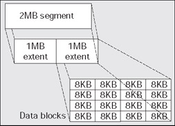
Segments themselves consist of one or more extent. An extent is a contiguous allocation of space in a file. Every segment starts with at least one extent and some objects may require at least two (rollback segments are an example of a segment that require at least two extents). In order for an object to grow beyond its initial extent, it will request another extent be allocated to it. This second extent will not necessarily be right next to the first extent on disk, it may very well not even be allocated in the same file as the first extent. It may be located very far away from it, but the space within an extent is always contiguous in a file. Extents vary in size from one block to 2 GB in size.
Extents, in turn, consist of blocks. A block is the smallest unit of space allocation in Oracle. Blocks are where your rows of data, or index entries, or temporary sort results will be stored. A block is what Oracle generally reads and writes from and to disk. Blocks in Oracle are generally one of three common sizes - 2 KB, 4 KB, or 8 KB (although 16 KB and 32 KB are also permissible). The relationship between segments, extents, and blocks looks like this:
A segment is made up of one or more extents - an extent is a contiguous allocation of blocks.
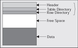
The block size for a database is a constant once the database is created - each and every block in the database will be the same size. All blocks have the same general format, which looks something like this:
The block header contains information about the type of block (a table block, index block, and so on), transaction information regarding active and past transactions on the block, and the address (location) of the block on the disk. The table directory, if present, contains information about the tables that store rows in this block (data from more than one table may be stored on the same block). The row directory contains information describing the rows that are to be found on the block. This is an array of pointers to where the rows are to be found in the data portion of the block. These three pieces of the block are collectively known as the block overhead - space used on the block that is not available for your data, but rather is used by Oracle to manage the block itself. The remaining two pieces of the block are rather straightforward - there will possibly be free space on a block and then there will generally be used space that is currently storing data.
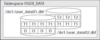
Now that we have a cursory understanding of segments, which consist of extents, which consist of blocks, we are ready to see what a tablespace is, and then how files fit into the picture. A tablespace is a container - it holds segments. Each and every segment belongs to exactly one tablespace. A tablespace may have many segments within it. All of the extents for a given segment will be found in the tablespace associated with that segment. Segments never cross tablespace boundaries. A tablespace itself has one or more data files associated with it. An extent for any given segment in a tablespace will be contained entirely within one data file. However, a segment may have extents from many different data files. Graphically it might look like this:
So, here we see tablespace named USER_DATA. It consists of two data files, user_data01, and user_data02. It has three segments allocated it, T1, T2, and I1 (probably two tables and an index). The tablespace has four extents allocated in it and each extent is depicted as a contiguous set of database blocks. Segment T1 consists of two extents, one extent in each file. Segment T2 and I1 each have one extent depicted. If we needed more space in this tablespace, we could either resize the data files already allocated to the tablespace, or we could add a third data file to it.
Tablespaces are a logical storage container in Oracle. As developers we will create segments in tablespaces. We will never get down to the raw 'file level' - we do not specify that we want our extents to be allocated in a specific file. Rather, we create objects in tablespaces and Oracle takes care of the rest. If at some point in the future, the DBA decides to move our data files around on disk to more evenly distribute I/O - that is OK with us. It will not affect our processing at all.
In summary, the hierarchy of storage in Oracle is as follows:
A database is made up of one or more tablespaces.
A tablespace is made up of one or more data files. A tablespace contains segments.
A segment (TABLE, INDEX, and so on) is made up of one or more extents. A segment exists in a tablespace, but may have data in many data files within that tablespace.
An extent is a contiguous set of blocks on disk. An extent is in a single tablespace and furthermore, is always in a single file within that tablespace.
A block is the smallest unit of allocation in the database. A block is the smallest unit of I/O used by a database.
Before we leave this topic of data files, we will look at one more topic to do with tablespaces. We will look at how extents are managed in a tablespace. Prior to Oracle 8.1.5, there was only one method to manage the allocation of extents within a tablespace. This method is called a dictionary-managed tablespace. That is, the space within a tablespace was managed in data dictionary tables, much in the same way you would manage accounting data, perhaps with a DEBIT and CREDIT table. On the debit side, we have all of the extents allocated to objects. On the credit side, we have all of the free extents available for use. When an object needed another extent, it would ask the system to get one. Oracle would then go to its data dictionary tables, run some queries, find the space (or not), and then update a row in one table (or remove it all together), and insert a row into another. Oracle managed space in very much the same way you will write your applications by modifying data, and moving it around.
This SQL, executed on your behalf in the background to get the additional space, is referred to as recursive SQL. Your SQL INSERT statement caused other recursive SQL to be executed to get more space. This recursive SQL could be quite expensive, if it is done frequently. Such updates to the data dictionary must be serialized; they cannot be done simultaneously. They are something to be avoided.
In earlier releases of Oracle, we would see this space management issue, this recursive SQL overhead, most often occurred in temporary tablespaces (this is before the introduction of 'real' temporary tablespaces). Space would frequently be allocated (we have to delete from one dictionary table and insert into another) and de-allocated (put the rows we just moved back where they were initially). These operations would tend to serialize, dramatically decreasing concurrency, and increasing wait times. In version 7.3, Oracle introduced the concept of a temporary tablespace to help alleviate this issue. A temporary tablespace was one in which you could create no permanent objects of your own. This was fundamentally the only difference; the space was still managed in the data dictionary tables. However, once an extent was allocated in a temporary tablespace, the system would hold onto it (would not give the space back). The next time someone requested space in the temporary tablespace for any purpose, Oracle would look for an already allocated extent in its memory set of allocated extents. If it found one there, it would simply reuse it, else it would allocate one the old fashioned way. In this fashion, once the database had been up and running for a while, the temporary segment would appear full but would actually just be 'allocated'. The free extents were all there; they were just being managed differently. When someone needed temporary space, Oracle would just look for that space in an in-memory data structure, instead of executing expensive, recursive SQL.
In Oracle 8.1.5 and later, Oracle goes a step further in reducing this space management overhead. They introduced the concept of a locally managed tablespace as opposed to a dictionary managed one. This effectively does for all tablespaces, what Oracle7.3 did for temporary tablespaces - it removes the need to use the data dictionary to manage space in a tablespace. With a locally managed tablespace, a bitmap stored in each data file is used to manage the extents. Now, to get an extent all the system needs to do is set a bit to 1 in the bitmap. To free space - set it back to 0. Compared to using dictionary-managed tablespaces, this is incredibly fast. We no longer serialize for a long running operation at the database level for space requests across all tablespaces. Rather, we serialize at the tablespace level for a very fast operation. Locally managed tablespaces have other nice attributes as well, such as the enforcement of a uniform extent size, but that is starting to get heavily into the role of the DBA.
Temp Files
Temporary data files (temp files) in Oracle are a special type of data file. Oracle will use temporary files to store the intermediate results of a large sort operation, or result set, when there is insufficient memory to hold it all in RAM. Permanent data objects, such as a table or an index, will never be stored in a temporary file, but the contents of a temporary table or index would be. So, you'll never create your application tables in a temporary data file, but you might store data there when you use a temporary table.
Temporary files are treated in a special way by Oracle. Normally, each and every change you make to an object will be recorded in the redo logs - these transaction logs can be replayed at a later date in order to 'redo a transaction'. We might do this during recovery from failure for example. Temporary files are excluded from this process. Temporary files never have redo generated for them, although they do have UNDO generated, when used for global temporary tables, in the event you decide to rollback some work you have done in your session. Your DBA never needs to back up a temporary data file, and in fact if they do they are only wasting their time, as you can never restore a temporary data file.
It is recommended that your database be configured with locally managed temporary tablespaces. You'll want to make sure your DBA uses a CREATETEMPORARYTABLESPACE command. You do not want them to just alter a permanent tablespace to a temporary one, as you do not get the benefits of temp files that way. Additionally, you'll want them to use a locally managed tablespace with uniform extent sizes that reflect your sort_area_size setting. Something such as:
As we are starting to get deep into DBA-related activities once again, we'll move onto the next topic.
Control Files
The control file is a fairly small file (it can grow up to 64 MB or so in extreme cases) that contains a directory of the other files Oracle needs. The parameter file (init.ora file) tells the instance where the control files are, the control files tell the instance where the database and online redo log files are. The control files also tell Oracle other things, such as information about checkpoints that have taken place, the name of the database (which should match the db_nameinit.ora parameter), the timestamp of the database as it was created, an archive redo log history (this can make a control file large in some cases), and so on.
Control files should be multiplexed either by hardware (RAID) or by Oracle when RAID or mirroring is not available - more than one copy of them should exist and they should be stored on separate disks, to avoid losing them in the event you have a disk failure. It is not fatal to lose your control files, it just makes recovery that much harder.
Control files are something a developer will probably never have to actually deal with. To a DBA they are an important part of the database, but to a software developer they are not extremely relevant.
Redo Log Files
Redo log files are extremely crucial to the Oracle database. These are the transaction logs for the database. They are used only for recovery purposes - their only purpose in life is to be used in the event of an instance or media failure, or as a method of maintaining a standby database for failover. If the power goes off on your database machine, causing an instance failure, Oracle will use the online redo logs in order to restore the system to exactly the point it was at immediately prior to the power outage. If your disk drive containing your datafile fails permanently, Oracle will utilize archived redo logs, as well as online redo logs, in order to recover a backup of that drive to the correct point in time. Additionally, if you 'accidentally' drop a table or remove some critical information and commit that operation, you can restore a backup and have Oracle restore it to the point immediately prior to the 'accident' using these online and archive redo log files.
Virtually every operation you perform in Oracle generates some amount of redo to be written to the online redo log files. When you insert a row into a table, the end result of that insert is written to the redo logs. When you delete a row, the fact that you deleted that row is written. When you drop a table, the effects of that drop are written to the redo log. The data from the table you dropped is not written; however the recursive SQL that Oracle performs to drop the table, does generate redo. For example, Oracle will delete a row from the SYS.OBJ$ table and this will generate redo.
Some operations may be performed in a mode that generates as little redo as possible. For example, I can create an index with the NOLOGGING attribute. This means that the initial creation of that index will not be logged, but any recursive SQL Oracle performs on my behalf will be. For example the insert of a row into SYS.OBJ$ representing the existence of the index will not be logged. All subsequent modifications of the index using SQL inserts, updates and deletes will however, be logged.
There are two types of redo log files that I've referred to - online and archived. We will take a look at each. In Chapter 5, Redo and Rollback, we will take another look at redo in conjunction with rollback segments, to see what impact they have on you the developer. For now, we will just concentrate on what they are and what purpose they provide.
Online Redo Log
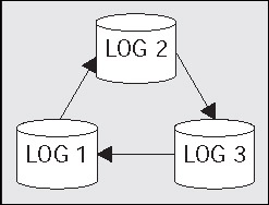
Every Oracle database has at least two online redo log files. These online redo log files are fixed in size and are used in a circular fashion. Oracle will write to log file 1, and when it gets to the end of this file, it will switch to log file 2, and rewrite the contents of that file from start to end. When it has filled log file 2, it will switch back to log file 1 (assuming we have only two redo log files, if you have three, it would of course proceed onto the third file):
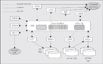
The act of switching from one log file to the other is called a log switch. It is important to note that a log switch may cause a temporary 'hang' in a poorly tuned database. Since the redo logs are used to recover transactions in the event of a failure, we must assure ourselves that we won't need the contents of a redo log file in the event of a failure before we reuse it. If Oracle is not sure that it won't need the contents of a log file, it will suspend operations in the database momentarily, and make sure that the data this redo 'protects' is safely on disk itself. Once it is sure of that, processing will resume and the redo file will be reused. What we've just started to talk about here is a key database concept - checkpointing. In order to understand how online redo logs are used, we'll need to know something about checkpointing, how the database buffer cache works, and what a process called Database Block Writer (DBWn) does. The database buffer cache and DBWn are covered in more detail a little later on, but we will skip ahead a little anyway and touch on them now.
The database buffer cache is where database blocks are stored temporarily. This is a structure in the SGA of Oracle. As blocks are read, they are stored in this cache - hopefully to allow us to not have to physically re-read them later. The buffer cache is first and foremost a performance-tuning device, it exists solely to make the very slow process of physical I/O appear to be much faster then it is. When we modify a block by updating a row on it, these modifications are done in memory, to the blocks in the buffer cache. Enough information to redo this modification is stored in the redo log buffer, another SGA data structure. When you COMMIT your modifications, making them permanent, Oracle does not go to all of the blocks you modified in the SGA and write them to disk. Rather, it just writes the contents of the redo log buffer out to the online redo logs. As long as that modified block is in the buffer cache and is not on disk, we need the contents of that online redo log in the event the database fails. If at the instant after we committed, the power was turned off, the database buffer cache would be wiped out.
If this happens, the only record of our change is in that redo log file. Upon restart of the database, Oracle will actually replay our transaction, modifying the block again in the same way we did, and committing it for us. So, as long as that modified block is cached and not written to disk, we cannot reuse that redo log file.
This is where DBWn comes into play. It is the Oracle background process that is responsible for making space in the buffer cache when it fills up and, more importantly, for performing checkpoints. A checkpoint is the flushing of dirty (modified) blocks from the buffer cache to disk. Oracle does this in the background for us. Many things can cause a checkpoint to occur, the most common event being a redo log switch. As we filled up log file 1 and switched to log file 2, Oracle initiated a checkpoint. At this point in time, DBWn started flushing to disk all of the dirty blocks that are protected by log file 1. Until DBWn flushes all of these blocks protected by that log file, Oracle cannot reuse it. If we attempt to use it before DBWn has finished its checkpoint, we will get a message like this:
...Thread 1 cannot allocate new log, sequence 66Checkpoint not complete Current log# 2 seq# 65 mem# 0: C:\ORACLE\ORADATA\TKYTE816\REDO02.LOG...
In our databases ALERT log (the alert log is a file on the server that contains informative messages from the server such as startup and shutdown messages, and exceptional events, such as an incomplete checkpoint). So, at this point in time, when this message appeared, processing was suspended in the database while DBWn hurriedly finished its checkpoint. Oracle gave all the processing power it could, to DBWn at that point in the hope it would finish faster.
This is a message you never want to see in a nicely tuned database instance. If you do see it, you know for a fact that you have introduced artificial, unnecessary waits for your end users. This can always be avoided. The goal (and this is for the DBA, not the developer necessarily) is to have enough online redo log files allocated so that you never attempt to reuse a log file before the checkpoint initiated by it completes. If you see this message frequently, it means your DBA has not allocated sufficient online redo logs for your application, or that DBWn needs to be tuned to work more efficiently. Different applications will generate different amounts of redo log. A DSS (Decision Support System, query only) system will naturally generate significantly less online redo log then an OLTP (transaction processing) system would. A system that does a lot of image manipulation in BLOBs (Binary Large OBjects) in the database may generate radically more redo then a simple order entry system. An order entry system with 100 users will probably generate a tenth the amount of redo 1,000 users would generate. There is no 'right' size for your redo logs, although you do want to ensure they are large enough.
There are many things you must take into consideration when setting both the size of, and the number of, online redo logs. Many of them are out of the scope of this particular book, but I'll list some of them to give you an idea:
Standby database - If you are utilizing the standby database feature, whereby redo logs are sent to another machine after they are filled and applied to a copy of your database, you will most likely want lots of small redo log files. This will help ensure the standby database is never too far out of sync with the primary database.
Lots of users modifying the same blocks - Here you might want large redo log files. Since everyone is modifying the same blocks, we would like to update them as many times as possible before writing them out to disk. Each log switch will fire a checkpoint so we would like to switch logs infrequently. This may, however, affect your recovery time.
Mean time to recover - If you must ensure that a recovery takes as little time as possible, you may be swayed towards smaller redo log files, even if the previous point is true. It will take less time to process one or two small redo log files than one gargantuan one upon recovery. The overall system will run slower than it absolutely could day-to-day perhaps (due to excessive checkpointing), but the amount of time spent in recovery will be smaller. There are other database parameters that may also be used to reduce this recovery time, as an alternative to the use of small redo log files.
Archived Redo Log
The Oracle database can run in one of two modes - NOARCHIVELOG mode and ARCHIVELOG mode. I believe that a system is not a production system unless it is in ARCHIVELOG mode. A database that is not in ARCHIVELOG mode will, some day, lose data. It is inevitable; you will lose data if you are not in ARCHIVELOG mode. Only a test or development system should execute in NOARCHIVELOG mode.
The difference between these two modes is simply what happens to a redo log file when Oracle goes to reuse it. 'Will we keep a copy of that redo or should Oracle just overwrite it, losing it forever?' It is an important question to answer. Unless you keep this file, we cannot recover data from a backup to the current point in time. Say you take a backup once a week on Saturday. Now, on Friday afternoon, after you have generated hundreds of redo logs over the week, your hard disk fails. If you have not been running in ARCHIVELOG mode, the only choices you have right now are:
Drop the tablespace(s) associated with the failed disk. Any tablespace that had a file on that disk must be dropped, including the contents of that tablespace. If the SYSTEM tablespace (Oracle's data dictionary) is affected, you cannot do this.
Restore last Saturday's data and lose all of the work you did that week.
Neither option is very appealing. Both imply that you lose data. If you had been executing in ARCHIVELOG mode on the other hand, you simply would have found another disk. You would have restored the affected files from Saturday's backup onto it. Lastly, you would have applied the archived redo logs, and ultimately, the online redo logs to them (in effect replay the weeks worth of transactions in fast forward mode). You lose nothing. The data is restored to the point in time of the failure.
People frequently tell me they don't need ARCHIVELOG mode for their production systems. I have yet to meet anyone who was correct in that statement. Unless they are willing to lose data some day, they must be in ARCHIVELOG mode. 'We are using RAID-5, we are totally protected' is a common excuse. I've seen cases where, due to a manufacturing error, all five disks in a raid set froze, all at the same time. I've seen cases where the hardware controller introduced corruption into the data files, so they safely protected corrupt data. If we had the backups from before the hardware failure, and the archives were not affected, we could have recovered. The bottom line is that there is no excuse for not being in ARCHIVELOG mode on a system where the data is of any value. Performance is no excuse - properly configured archiving adds little overhead. This and the fact that a 'fast system' that 'loses data' is useless, would make it so that even if archiving added 100 percent overhead, you would need to do it.
Don't let anyone talk you out of being in ARCHIVELOG mode. You spent a long time developing your application, so you want people to trust it. Losing their data will not instill confidence in them.
Files Wrap-Up
Here we have explored the important types of files used by the Oracle database, from lowly parameter files (without which you won't even be able to get started), to the all important redo log and data files. We have explored the storage structures of Oracle from tablespaces to segments, and then extents, and finally down to database blocks, the smallest unit of storage. We have reviewed how checkpointing works in the database, and even started to look ahead at what some of the physical processes or threads of Oracle do. In later components of this chapter, we'll take a much more in depth look at these processes and memory structures.
The Memory Structures
Now we are ready to look at Oracle's major memory structures. There are three major memory structures to be considered:
SGA, System Global Area - This is a large, shared memory segment that virtually all Oracle processes will access at one point or another.
PGA, Process Global Area - This is memory, which is private to a single process or thread, and is not accessible from other processes/threads.
UGA, User Global Area - This is memory associated with your session. It will be found either in the SGA or the PGA depending on whether you are running in MTS mode (then it'll be in the SGA), or dedicated server (it'll be in the PGA).
We will briefly discuss the PGA and UGA, and then move onto the really big structure, the SGA.
PGA and UGA
As stated earlier, the PGA is a process piece of memory. This is memory specific to a single operating system process or thread. This memory is not accessible by any other process/thread in the system. It is typically allocated via the C run-time call malloc(), and may grow (and shrink even) at run-time. The PGA is never allocated out of Oracle's SGA - it is always allocated locally by the process or thread.
The UGA is in effect, your session's state. It is memory that your session must always be able to get to. The location of the UGA is wholly dependent on how Oracle has been configured to accept connections. If you have configured MTS, then the UGA must be stored in a memory structure that everyone has access to - and that would be the SGA. In this way, your session can use any one of the shared servers, since any one of them can read and write your sessions data. On the other hand, if you are using a dedicated server connection, this need for universal access to your session state goes away, and the UGA becomes virtually synonymous with the PGA - it will in fact be contained in the PGA. When you look at the system statistics, you'll find the UGA reported in the PGA in dedicated server mode (the PGA will be greater than, or equal to, the UGA memory used; the PGA memory size will include the UGA size as well).
One of the largest impacts on the size of your PGA/UGA will be the init.ora or session-level parameters, SORT_AREA_SIZE and SORT_AREA_RETAINED_SIZE. These two parameters control the amount of space Oracle will use to sort data before writing it to disk, and how much of that memory segment will be retained after the sort is done. The SORT_AREA_SIZE is generally allocated out of your PGA and the SORT_AREA_RETAINED_SIZE will be in your UGA. We can monitor the size of the UGA/PGA by querying a special Oracle V$ table, also referred to as a dynamic performance table. We'll find out more about these V$ tables in Chapter 10, Tuning Strategies and Tools. Using these V$ tables, we can discover our current usage of PGA and UGA memory. For example, I'll run a small test that will involve sorting lots of data. We'll look at the first couple of rows and then discard the result set. We can look at the 'before' and 'after' memory usage:
tkyte@TKYTE816> select a.name, b.value 2 from v$statname a, v$mystat b 3 where a.statistic# = b.statistic# 4 and a.name like '%ga %' 5 /NAME VALUE------------------------------ ----------session uga memory 67532session uga memory max 71972session pga memory 144688session pga memory max 1446884 rows selected.
So, before we begin we can see that we have about 70 KB of data in the UGA and 140 KB of data in the PGA. The first question is, how much memory are we using between the PGA and UGA? It is a trick question, and one that you cannot answer unless you know if we are connected via a dedicated server or a shared server over MTS, and even then it might be hard to figure out. In dedicated server mode, the UGA is totally contained within the PGA. There, we would be consuming 140 KB of memory in our process or thread. In MTS mode, the UGA is allocated from the SGA, and the PGA is in the shared server. So, in MTS mode, by the time we get the last row from the above query, our process may be in use by someone else. That PGA isn't 'ours', so technically we are using 70 KB of memory (except when we are actually running the query at which point we are using 210 KB of memory between the combined PGA and UGA).
Now we will do a little bit of work and see what happens with our PGA/UGA:
tkyte@TKYTE816> show parameter sort_areaNAME TYPE VALUE------------------------------------ ------- ------------------------------sort_area_retained_size integer 65536sort_area_size integer 65536tkyte@TKYTE816> set pagesize 10tkyte@TKYTE816> set pause ontkyte@TKYTE816> select * from all_objects order by 1, 2, 3, 4;...(control C after first page of data) ...tkyte@TKYTE816> set pause offtkyte@TKYTE816> select a.name, b.value 2 from v$statname a, v$mystat b 3 where a.statistic# = b.statistic# 4 and a.name like '%ga %' 5 /NAME VALUE------------------------------ ----------session uga memory 67524session uga memory max 174968session pga memory 291336session pga memory max 2913364 rows selected.
As you can see, our memory usage went up - we've done some sorting of data. Our UGA temporarily increased by about the size of SORT_AREA_RETAINED_SIZE while our PGA went up a little more. In order to perform the query and the sort (and so on), Oracle allocated some additional structures that our session will keep around for other queries. Now, let's retry that operation but play around with the size of our SORT_AREA:
tkyte@TKYTE816> alter session set sort_area_size=1000000;Session altered.tkyte@TKYTE816> select a.name, b.value 2 from v$statname a, v$mystat b 3 where a.statistic# = b.statistic# 4 and a.name like '%ga %' 5 /NAME VALUE------------------------------ ----------session uga memory 63288session uga memory max 174968session pga memory 291336session pga memory max 2913364 rows selected.tkyte@TKYTE816> show parameter sort_areaNAME TYPE VALUE------------------------------------ ------- ------------------------------sort_area_retained_size integer 65536sort_area_size integer 1000000tkyte@TKYTE816> select * from all_objects order by 1, 2, 3, 4;...(control C after first page of data) ...tkyte@TKYTE816> set pause offtkyte@TKYTE816> select a.name, b.value 2 from v$statname a, v$mystat b 3 where a.statistic# = b.statistic# 4 and a.name like '%ga %' 5 /NAME VALUE------------------------------ ----------session uga memory 67528session uga memory max 174968session pga memory 1307580session pga memory max 13075804 rows selected.
As you can see, our PGA has grown considerably this time. By about the 1,000,000 bytes of SORT_AREA_SIZE we are using. It is interesting to note that the UGA did not move at all in this case. We can change that by altering the SORT_AREA_RETAINED_SIZE as follows:
tkyte@TKYTE816> alter session set sort_area_retained_size=1000000;Session altered.tkyte@TKYTE816> select a.name, b.value 2 from v$statname a, v$mystat b 3 where a.statistic# = b.statistic# 4 and a.name like '%ga %' 5 /NAME VALUE------------------------------ ----------session uga memory 63288session uga memory max 174968session pga memory 1307580session pga memory max 13075804 rows selected.tkyte@TKYTE816> show parameter sort_areaNAME TYPE VALUE------------------------------------ ------- ------------------------------sort_area_retained_size integer 1000000sort_area_size integer 1000000tkyte@TKYTE816> select * from all_objects order by 1, 2, 3, 4;...(control C after first page of data) ...tkyte@TKYTE816> select a.name, b.value 2 from v$statname a, v$mystat b 3 where a.statistic# = b.statistic# 4 and a.name like '%ga %' 5 /NAME VALUE------------------------------ ----------session uga memory 66344session uga memory max 1086120session pga memory 1469192session pga memory max 14691924 rows selected.
Here, we see that our UGA memory max shot way up - to include the SORT_AREA_RETAINED_SIZE amount of data, in fact. During the processing of our query, we had a 1 MB of sort data 'in memory cache'. The rest of the data was on disk in a temporary segment somewhere. After our query completed execution, this memory was given back for use elsewhere. Notice how PGA memory does not shrink back. This is to be expected as the PGA is managed as a heap and is created via malloc()'ed memory. Some processes within Oracle will explicitly free PGA memory - others allow it to remain in the heap (sort space for example stays in the heap). The shrinking of a heap like this typically does nothing (processes tend to grow in size, not to shrink). Since the UGA is a 'sub-heap' (the 'parent' heap being either the PGA or SGA) it is made to shrink. If we wish, we can force the PGA to shrink:
tkyte@TKYTE816> exec dbms_session.free_unused_user_memory;PL/SQL procedure successfully completed.tkyte@TKYTE816> select a.name, b.value 2 from v$statname a, v$mystat b 3 where a.statistic# = b.statistic# 4 and a.name like '%ga %' 5 /NAME VALUE------------------------------ ----------session uga memory 73748session uga memory max 1086120session pga memory 183360session pga memory max 1469192
However, you should be aware that on most systems, this is somewhat a waste of time. You may have shrunk the size of the PGA heap as far as Oracle is concerned, but you haven't really given the OS any memory back in most cases. In fact, depending on the OS method of managing memory, you may actually be using more memory in total according to the OS. It will all depend on how malloc(), free(), realloc(), brk(), and sbrk() (the C memory management routines) are implemented on your platform.
So, here we have looked at the two memory structures, the PGA and the UGA. We understand now that the PGA is private to a process. It is the set of variables that an Oracle dedicated or shared server needs to have independent of a session. The PGA is a 'heap' of memory in which other structures may be allocated. The UGA on the other hand, is also a heap of memory in which various session-specific structures may be defined. The UGA is allocated from the PGA when you use the dedicated server mode to connect to Oracle, and from the SGA in MTS mode. This implies that when using MTS, you must size your SGA to have enough UGA space in it to cater for every possible user that will ever connect to your database concurrently. So, the SGA of a database running MTS is generally much larger than the SGA for a similarly configured, dedicated server mode only, database.
SGA
Every Oracle instance has one big memory structure collectively referred to as the SGA, the System Global Area. This is a large, shared memory structure that every Oracle process will access at one point or another. It will vary from a couple of MBs on small test systems to hundreds of MBs on medium to large systems, and into many GBs in size for really big systems.
On a UNIX operating system, the SGA is a physical entity that you can 'see' from the operating system command line. It is physically implemented as a shared memory segment - a standalone piece of memory that processes may attach to. It is possible to have an SGA on a system without having any Oracle processes; the memory stands alone. It should be noted however that if you have an SGA without any Oracle processes, it indicates that the database crashed in some fashion. It is not a normal situation but it can happen. This is what an SGA 'looks' like on UNIX:
$ ipcs -mbIPC status from <running system> as of Mon Feb 19 14:48:26 EST 2001T ID KEY MODE OWNER GROUP SEGSZShared Memory:m 105 0xf223dfc8 --rw-r----- ora816 dba 186802176
On Windows, you really cannot see the SGA as you can in UNIX. Since Oracle executes as a single process with a single address space on that platform, the SGA is allocated as private memory to the ORACLE.EXE process. If you use the Windows Task Manager or some other performance tool, you can see how much memory ORACLE.EXE has allocated, but you cannot see what is the SGA versus any other piece of allocated memory.
Within Oracle itself we can see the SGA regardless of platform. There is another magic V$ table called V$SGASTAT. It might look like this:
tkyte@TKYTE816> compute sum of bytes on pooltkyte@TKYTE816> break on pool skip 1tkyte@TKYTE816> select pool, name, bytes 2 from v$sgastat 3 order by pool, name;POOL NAME BYTES----------- ------------------------------ ----------java pool free memory 18366464 memory in use 2605056*********** ----------sum 20971520large pool free memory 6079520 session heap 64480*********** ----------sum 6144000shared pool Checkpoint queue 73764 KGFF heap 5900 KGK heap 17556 KQLS heap 554560 PL/SQL DIANA 364292 PL/SQL MPCODE 138396 PLS non-lib hp 2096 SYSTEM PARAMETERS 61856 State objects 125464 VIRTUAL CIRCUITS 97752 character set object 58936 db_block_buffers 408000 db_block_hash_buckets 179128 db_files 370988 dictionary cache 319604 distributed_transactions- 180152 dlo fib struct 40980 enqueue_resources 94176 event statistics per sess 201600 file # translation table 65572 fixed allocation callback 320 free memory 9973964 joxlod: in ehe 52556 joxlod: in phe 4144 joxs heap init 356 library cache 1403012 message pool freequeue 231152 miscellaneous 562744 processes 40000 sessions 127920 sql area 2115092 table columns 19812 transaction_branches 368000 transactions 58872 trigger defini 2792 trigger inform 520*********** ----------sum 18322028 db_block_buffers 24576000 fixed_sga 70924 log_buffer 66560*********** ----------sum 2471348443 rows selected.
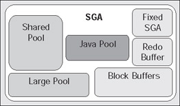
The SGA is broken up into various pools. They are:
Java pool - The Java pool is a fixed amount of memory allocated for the JVM running in the database.
Large pool - The large pool is used by the MTS for session memory, by Parallel Execution for message buffers, and by RMAN Backup for disk I/O buffers.
Shared pool - The shared pool contains shared cursors, stored procedures, state objects, dictionary caches, and many dozens of other bits of data.
The 'Null' pool - This one doesn't really have a name. It is the memory dedicated to block buffers (cached database blocks), the redo log buffer and a 'fixed SGA' area.
So, an SGA might look like this:
The init.ora parameters that have the most effect on the overall size of the SGA are:
JAVA_POOL_SIZE - controls the size of the Java pool.
SHARED_POOL_SIZE - controls the size of the shared pool, to some degree.
LARGE_POOL_SIZE - controls the size of the large pool.
DB_BLOCK_BUFFERS - controls the size of the block buffer cache.
LOG_BUFFER - controls the size of the redo buffer to some degree.
With the exception of the SHARED_POOL_SIZE and LOG_BUFFER, there is a one-to-one correspondence between the init.ora parameters, and the amount of memory allocated in the SGA. For example, if you multiply DB_BLOCK_BUFFERS by your databases block size, you'll typically get the size of the DB_BLOCK_BUFFERS row from the NULL pool in V$SGASTAT (there is some overhead added for latches). If you look at the sum of the bytes from V$SGASTAT for the large pool, this will be the same as the LARGE_POOL_SIZE parameter.
Fixed SGA
The fixed SGA is a component of the SGA that varies in size from platform to platform and release to release. It is 'compiled' into the Oracle binary itself at installation time (hence the name 'fixed'). The fixed SGA contains a set of variables that point to the other components of the SGA, and variables that contain the values of various parameters. The size of the fixed SGA is something over which we have no control, and it is generally very small. Think of this area as a 'bootstrap' section of the SGA, something Oracle uses internally to find the other bits and pieces of the SGA.
Redo Buffer
The redo buffer is where data that needs to be written to the online redo logs will be cached temporarily before it is written to disk. Since a memory-to-memory transfer is much faster then a memory to disk transfer, use of the redo log buffer can speed up operation of the database. The data will not reside in the redo buffer for a very long time. In fact, the contents of this area are flushed:
Every three seconds, or
Whenever someone commits, or
When it gets one third full or contains 1 MB of cached redo log data.
For these reasons, having a redo buffer in the order of many tens of MB in size is typically just a waste of good memory. In order to use a redo buffer cache of 6 MB for example, you would have to have very long running transactions that generate 2 MB of redo log every three seconds or less. If anyone in your system commits during that three-second period of time, you will never use the 2MB of redo log space; it'll continuously be flushed. It will be a very rare system that will benefit from a redo buffer of more than a couple of megabytes in size.
The default size of the redo buffer, as controlled by the LOG_BUFFERinit.ora parameter, is the greater of 512 KB and (128 * number of CPUs) KB. The minimum size of this area is four times the size of the largest database block size supported on that platform. If you would like to find out what that is, just set your LOG_BUFFERS to 1 byte and restart your database. For example, on my Windows 2000 instance I see:
SVRMGR> show parameter log_bufferNAME TYPE VALUE----------------------------------- ------- ------------------------------log_buffer integer 1SVRMGR> select * from v$sgastat where name = 'log_buffer';POOL NAME BYTES----------- -------------------------- ---------- log_buffer 66560
The smallest log buffer I can really have, regardless of my init.ora settings, is going to be 65 KB. In actuality - it is a little larger then that:
tkyte@TKYTE816> select * from v$sga where name = 'Redo Buffers';NAME VALUE------------------------------ ----------Redo Buffers 77824
It is 76 KB in size. This extra space is allocated as a safety device - as 'guard' pages to protect the redo log buffer pages themselves.
Block Buffer Cache
So far, we have looked at relatively small components of the SGA. Now we are going to look at one that is possibly huge in size. The block buffer cache is where Oracle will store database blocks before writing them to disk, and after reading them in from disk. This is a crucial area of the SGA for us. Make it too small and our queries will take forever to run. Make it too big and we'll starve other processes (for example, you will not leave enough room for a dedicated server to create its PGA and you won't even get started).
The blocks in the buffer cache are basically managed in two different lists. There is a 'dirty' list of blocks that need to be written by the database block writer (DBWn - we'll be taking a look at that process a little later). Then there is a list of 'not dirty' blocks. This used to be a LRU (Least Recently Used) list in Oracle 8.0 and before. Blocks were listed in order of use. The algorithm has been modified slightly in Oracle 8i and in later versions. Instead of maintaining the list of blocks in some physical order, Oracle employs a 'touch count' schema. This effectively increments a counter associated with a block every time you hit it in the cache. We can see this in one of the truly magic tables, the X$ tables. These X$ tables are wholly undocumented by Oracle, but information about them leaks out from time to time.
The X$BH table shows information about the blocks in the block buffer cache. Here, we can see the 'touch count' get incremented as we hit blocks. First, we need to find a block. We'll use the one in the DUAL table, a special table with one row and one column that is found in all Oracle databases. We need to know the file number and block number for that block:
tkyte@TKYTE816> select file_id, block_id 2 from dba_extents 3 where segment_name = 'DUAL' and owner = 'SYS'; FILE_ID BLOCK_ID---------- ---------- 1 465
Now we can use that information to see the 'touch count' on that block:
sys@TKYTE816> select tch from x$bh where file# = 1 and dbablk = 465; TCH---------- 10sys@TKYTE816> select * from dual;D-Xsys@TKYTE816> select tch from x$bh where file# = 1 and dbablk = 465; TCH---------- 11sys@TKYTE816> select * from dual;D-Xsys@TKYTE816> select tch from x$bh where file# = 1 and dbablk = 465; TCH---------- 12
Every time I touch that block, the counter goes up. A buffer no longer moves to the head of the list as it is used, rather it stays where it is in the list, and has its 'touch count' incremented. Blocks will naturally tend to move in the list over time however, because blocks are taken out of the list and put into the dirty list (to be written to disk by DBWn). Also, as they are reused, when the buffer cache is effectively full, and some block with a small 'touch count' is taken out of the list, it will be placed back into approximately the middle of the list with the new data. The whole algorithm used to manage these lists is fairly complex and changes subtly from release to release of Oracle as improvements are made. The actual full details are not relevant to us as developers, beyond the fact that heavily used blocks will be cached and blocks that are not used heavily will not be cached for long.
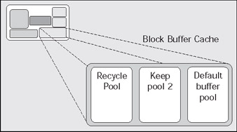
The block buffer cache, in versions prior to Oracle 8.0, was one big buffer cache. Every block was cached alongside every other block - there was no way to segment or divide up the space in the block buffer cache. Oracle 8.0 added a feature called multiple buffer pools to give us this ability. Using the multiple buffer pool feature, we can set aside a given amount of space in the block buffer cache for a specific segment or segments (segments as you recall, are indexes, tables, and so on). Now, we could carve out a space, a buffer pool, large enough to hold our 'lookup' tables in memory, for example. When Oracle reads blocks from these tables, they always get cached in this special pool. They will compete for space in this pool only with other segments targeted towards this pool. The rest of the segments in the system will compete for space in the default buffer pool. This will increase the likelihood of their staying in the cache and not getting aged out by other unrelated blocks. A buffer pool that is set up to cache blocks like this is known as a KEEP pool. The blocks in the KEEP pool are managed much like blocks in the generic block buffer cache described above - if you use a block frequently, it'll stay cached. If you do not touch a block for a while, and the buffer pool runs out of room, that block will be aged out of the pool.
We also have the ability to carve out a space for segments in the buffer pool. This space is called a RECYCLE pool. Here, the aging of blocks is done differently to the KEEP pool. In the KEEP pool, the goal is to keep 'warm' and 'hot' blocks cached for as long as possible. In the recycle pool, the goal is to age out a block as soon as it is no longer needed. This is advantageous for 'large' tables (remember, large is always relative, there is no absolute size we can put on 'large') that are read in a very random fashion. If the probability that a block will ever be re-read in a reasonable amount of time, there is no use in keeping this block cached for very long. Therefore, in a RECYCLE pool, things move in and out on a more regular basis.
So, taking the diagram of the SGA a step further, we can break it down to:
Shared Pool
The shared pool is one of the most critical pieces of memory in the SGA, especially in regards to performance and scalability. A shared pool that is too small can kill performance to the point where the system appears to hang. A shared pool that is too large can do the same thing. A shared pool that is used incorrectly will be a disaster as well.
So, what exactly is the shared pool? The shared pool is where Oracle caches many bits of 'program' data. When we parse a query, the results of that are cached here. Before we go through the job of parsing an entire query, Oracle searches here to see if the work has already been done. PL/SQL code that you run is cached here, so the next time you run it, Oracle doesn't have to read it in from disk again. PL/SQL code is not only cached here, it is shared here as well. If you have 1000 sessions all executing the same code, only one copy of the code is loaded and shared amongst all sessions. Oracle stores the system parameters in the shared pool. The data dictionary cache, cached information about database objects, is stored here. In short, everything but the kitchen sink is stored in the shared pool.
The shared pool is characterized by lots of small (4 KB or thereabouts) chunks of memory. The memory in the shared pool is managed on a LRU basis. It is similar to the buffer cache in that respect - if you don't use it, you'll lose it. There is a supplied package, DBMS_SHARED_POOL, which may be used to change this behavior - to forcibly pin objects in the shared pool. You can use this procedure to load up your frequently used procedures and packages at database startup time, and make it so they are not subject to aging out. Normally though, if over time a piece of memory in the shared pool is not reused, it will become subject to aging out. Even PL/SQL code, which can be rather large, is managed in a paging mechanism so that when you execute code in a very large package, only the code that is needed is loaded into the shared pool in small chunks. If you don't use it for an extended period of time, it will be aged out if the shared pool fills up and space is needed for other objects.
The easiest way to break Oracle's shared pool is to not use bind variables. As we saw in Chapter 1 on Developing Successful Oracle Applications, not using bind variables can bring a system to its knees for two reasons:
The system spends an exorbitant amount of CPU time parsing queries.
The system expends an extremely large amount of resources managing the objects in the shared pool as a result of never reusing queries.
If every query submitted to Oracle is a unique query with the values hard-coded, the concept of the shared pool is substantially defeated. The shared pool was designed so that query plans would be used over and over again. If every query is a brand new, never before seen query, then caching only adds overhead. The shared pool becomes something that inhibits performance. A common, misguided technique that many try in order to solve this issue is to add more space to the shared pool, but this typically only makes things worse than before. As the shared pool inevitably fills up once again, it gets to be even more of an overhead than the smaller shared pool, for the simple reason that managing a big, full-shared pool takes more work than managing a smaller full-shared pool.
The only true solution to this problem is to utilize shared SQL - to reuse queries. Later, in Chapter 10 on Tuning Strategies and Tools, we will take a look at the init.ora parameter CURSOR_SHARING that can work as a short term 'crutch' in this area, but the only real way to solve this issue is to use reusable SQL in the first place. Even on the largest of large systems, I find that there are at most 10,000 to 20,000 unique SQL statements. Most systems execute only a few hundred unique queries.
The following real-world example demonstrates just how bad things can get if you use of the shared pool poorly. I was asked to work on a system where the standard operating procedure was to shut down the database each and every night, in order to wipe out the SGA, and restart it clean. The reason for doing this was that the system was having issues during the day whereby it was totally CPU-bound and, if the database were left to run for more than a day, performance would really start to decline. This was solely due to the fact that, in the time period from 9am to 5pm, they would fill a 1 GB shared pool inside of a 1.1 GB SGA. This is true - 0.1 GB dedicated to block buffer cache and other elements, and 1 GB dedicated to caching unique queries that would never be executed again. The reason for the cold start was that if they left the system running for more than a day, they would run out of free memory in the shared pool. At that point, the overhead of aging structures out (especially from a structure so large) was such that it overwhelmed the system and performance was massively degraded (not that performance was that great anyway, since they were managing a 1 GB shared pool). Additionally, the people working on this system constantly wanted to add more and more CPUs to the machine, due to the fact that hard parsing SQL is so CPU-intensive. By correcting the application, allowing it to use bind variables, not only did the physical machine requirements drop (they then had many times more CPU power then they needed), the memory utilization was reversed. Instead of a 1 GB shared pool, they had less then 100 MB allocated - and never used it all over many weeks of continuous uptime.
One last comment about the shared pool and the init.ora parameter, SHARED_POOL_SIZE. There is no relationship between the outcome of the query:
sys@TKYTE816> select sum(bytes) from v$sgastat where pool = 'shared pool';SUM(BYTES)---------- 183220281 row selected.
and the SHARED_POOL_SIZEinit.ora parameter:
sys@TKYTE816> show parameter shared_pool_sizeNAME TYPE VALUE----------------------------------- ------- ------------------------------shared_pool_size string 15360000SVRMGR>
other than the fact that the SUM(BYTES)FROMV$SGASTAT will always be larger than the SHARED_POOL_SIZE. The shared pool holds many other structures that are outside the scope of the corresponding init.ora parameter. The SHARED_POOL_SIZE is typically the largest contributor to the shared pool as reported by the SUM(BYTES), but it is not the only contributor. For example, the init.ora parameter, CONTROL_FILES, contributes 264 bytes per file to the 'miscellaneous' section of the shared pool. It is unfortunate that the 'shared pool' in V$SGASTAT and the init.ora parameter SHARED_POOL_SIZE are named as they are, since the init.ora parameter contributes to the size of the shared pool, but it is not the only contributor.
Large Pool
The large pool is not so named because it is a 'large' structure (although it may very well be large in size). It is so named because it is used for allocations of large pieces of memory, bigger than the shared pool is designed to handle. Prior to its introduction in Oracle 8.0, all memory allocation took place in the shared pool. This was unfortunate if you were using features that made use of 'large' memory allocations such as MTS. This issue was further confounded by the fact that processing, which tended to need a lot of memory allocation, would use the memory in a different manner to the way in which the shared pool managed it. The shared pool manages memory in a LRU basis, which is perfect for caching and reusing data. Large memory allocations, however, tended to get a chunk of memory, use it, and then were done with it - there was no need to cache this memory.
What Oracle needed was something similar to the RECYCLE and KEEP buffer pools implemented for the block buffer cache. This is exactly what the large pool and shared pool are now. The large pool is a RECYCLE-style memory space whereas the shared pool is more like the KEEP buffer pool - if people appear to be using something frequently, then you keep it cached.
Memory allocated in the large pool is managed in a heap, much in the way C manages memory via malloc() and free(). As soon as you 'free' a chunk of memory, it can be used by other processes. In the shared pool, there really was no concept of 'freeing' a chunk of memory. You would allocate memory, use it, and then stop using it. After a while, if that memory needed to be reused, Oracle would age out your chunk of memory. The problem with using just a shared pool is that one size doesn't always fit all.
The large pool is used specifically by:
MTS - to allocate the UGA region in the SGA.
Parallel Execution of statements - to allow for the allocation of inter-process message buffers, used to coordinate the parallel query servers.
Backup - for RMAN disk I/O buffers.
As you can see, none of the above memory allocations should be managed in an LRU buffer pool designed to manage small chunks of memory. With MTS memory, for example, once a session logs out, this memory is never going to be reused so it should be immediately returned to the pool. Also, MTS memory tends to be 'large'. If you review our earlier examples, with the SORT_AREA_RETAINED_SIZE, the UGA can grow very large, and is definitely bigger than 4 KB chunks. Putting MTS memory into the shared pool causes it to fragment into odd sized pieces of memory and, furthermore you will find that large pieces of memory that will never be reused will age out memory that could be reused. This forces the database to do more work to rebuild that memory structure later.
The same is true for parallel query message buffers. Once they have delivered their message, they are no longer needed. Backup buffers, even more so - they are large, and once Oracle is done using them, they should just 'disappear'.
The large pool is not mandatory when using MTS, but it is highly recommended. If you do not have a large pool and use MTS, the allocations come out of the shared pool as they always did in Oracle 7.3 and before. This will definitely lead to degraded performance over some period of time, and should be avoided. The large pool will default to some size if either one of two init.ora parameters, DBWn_IO_SLAVES or PARALLEL_AUTOMATIC_TUNING are set. It is recommended that you set the size of the large pool manually yourself. The default mechanism is typically not the appropriate value for your situation.
Java Pool
The Java pool is the newest pool in the Oracle 8i database. It was added in version 8.1.5 to support the running of Java in the database. If you code a stored procedure in Java or put an EJB (Enterprise JavaBean) into the database, Oracle will make use of this chunk of memory when processing that code. An early quirk of the Java pool, in Oracle 8.1.5, was that it did not show up in the SHOWSGA command, and was not visible in V$SGASTAT view. This was particularly confusing at the time, since the JAVA_POOL_SIZEinit.ora parameter that controls the size of this structure defaults to 20 MB. This oversight had people wondering why their SGA was taking an extra 20 MB of RAM for the database.
As of version 8.1.6, however, the Java pool is visible in the V$SGASTAT view, as well as the variable size in the SHOWSGA command. The init.ora parameter JAVA_POOL_SIZE is used to fix the amount of memory allocated to the Java pool for all session-specific Java code and data. In Oracle 8.1.5, this parameter could take values from 1 MB to 1 GB. In Oracle 8.1.6 and later versions, the valid range of values is 32 KB to 1 GB in size. This is contrary to the documentation, which stills refers to the old minimum of 1 MB.
The Java pool is used in different ways, depending on the mode in which the Oracle server is running. In dedicated server mode, the Java pool includes the shared part of each Java class, which is actually used per session. These are basically the read-only parts (execution vectors, methods, and so on) and are about 4 to 8 KB per class.
Thus, in dedicated server mode (which will most likely be the case for applications using purely Java stored procedures), the total memory required for the Java pool is quite modest and can be determined based on the number of Java classes you will be using. It should be noted that none of the per-session state is stored in the SGA in dedicated server mode, as this information is stored in the UGA and, as you will recall, the UGA is included in the PGA in dedicated server mode.
When executing in MTS mode, the Java pool includes:
The shared part of each Java class, and
Some of the UGA used for per-session state of each session, which is allocated from the java_pool within the SGA. The remainder of the UGA will be located as normal in the shared pool, or if the large pool is configured it will be allocated there instead.
As the total size of the Java pool is fixed, application developers will need to estimate the total requirement of their applications, and multiply this by the number of concurrent sessions they need to support. This number will dictate the overall size of the Java pool. Each Java UGA will grow or shrink as needed, but bear in mind that the pool must be sized such that all UGAs combined must be able to fit in at the same time.
In MTS mode, which will be the case for applications using CORBA or EJBs (as pointed out in Chapter 1 on Developing Successful Oracle applications), the Java pool may need to be very large. Instead of being a function of the number of classes you use in your applications, it will be a function of the number of concurrent users. Just as the large pool could become very large under MTS, the Java pool may also become very large.
Memory Structures Wrap-Up
In this section, we have taken a look at the Oracle memory structure. We started at the process and session level, taking a look at the PGA (Process Global Area) and UGA (User Global Area), and their relationship to each other. We have seen how the mode in which you connect to Oracle will dictate how memory is organized. A dedicated server connection implies more memory used in the server process than under MTS, but that MTS implies there will be the need for a significantly larger SGA. Then, we discussed the components of the SGA itself, looking at its six main structures. We discovered the differences between the shared pool and the large pool, and looked at why you might want a large pool in order to 'save' your shared pool. We covered the Java pool and how it is used under various conditions. We looked at the block buffer cache and how that can be subdivided into smaller, more focused pools.
Now we are ready to move onto the physical processes that make up the rest of an Oracle instance.
The Processes
We have reached the last piece of the puzzle. We've investigated the database and the set of physical files that constitute a database. In covering the memory used by Oracle, we have looked at one half of an instance. The last remaining architectural issue is the set of processes that constitute the other half of the instance. Some of these processes, such as the database block writer (DBWn), and the log writer (LGWR) have cropped up already. Here, we will take a closer look at the function of each, what they do and why they do it. When we talk of 'process' here, it will be synonymous with 'thread' on operating systems where Oracle is implemented with threads. So, for example, when we talk about the DBWn process, the equivalent on windows is the DBWn thread.
There are three classes of processes in an Oracle instance:
Server Processes - These perform work based on a client's request. We have already looked at dedicated, and shared servers to some degree. These are the server processes.
Background Processes - These are the processes that start up with the database, and perform various maintenance tasks, such as writing blocks to disk, maintaining the online redo log, cleaning up aborted processes, and so on.
Slave Processes - These are similar to background processes but they are processes that perform extra work on behalf of either a background or a server process.
We will take a look at the processes in each of these three classes to see how they fit into the picture.
Server Processes
We briefly touched on these processes earlier in this section when we discussed dedicated and shared servers. Here, we will revisit the two server processes and review their architectures in more detail.
Both dedicated and shared servers have the same jobs - they process all of the SQL you give to them. When you submit a SELECT*FROMEMP query to the database, it is an Oracle dedicated/shared server that will parse the query, and place it into the shared pool (or find it in the shared pool already, hopefully). It is this process that will come up with the query plan. It is this process that will execute the query plan, perhaps finding the necessary data in the buffer cache, or reading the data from disk into the buffer cache. These server processes are the 'work horse' processes. Many times, you will find these processes to be the highest consumers of CPU time on your system, as they are the ones that do your sorting, your summing, your joining - pretty much everything.
In dedicated server mode, there will be a one-to-one mapping between a client session and a server process (or thread, as the case may be). If you have 100 sessions on a UNIX machine, there will be 100 processes executing on their behalf. Graphically it would look like this:
Your client application will have Oracle libraries linked into it. These libraries provide the Application Program Interface (API) that you need in order to talk to the database. These APIs know how to submit a query to the database, and process the cursor that is returned. They know how to bundle your requests into network calls that the dedicated server will know how to un-bundle. This piece of the picture is called Net8. This is the networking software/protocol that Oracle employs to allow for client server processing (even in a n-tier architecture, there is a client server program lurking). Oracle employs this same architecture even if Net8 is not technically involved in the picture. That is, when the client and server are on the same machine this two-process (also known as two-task) architecture is employed. This architecture provides two benefits:
Remote Execution - It is very natural for the client application to be executing on a machine other than the database itself.
Address Space Isolation - The server process has read-write access to the SGA. An errant pointer in a client process could easily corrupt data structures in the SGA, if the client process and server process were physically linked together.
Earlier in this chapter we saw how these dedicated servers are 'spawned' or created by the Oracle Net8 Listener process. We won't cover that process again, but rather we'll quickly look at what happens when the listener is not involved. The mechanism is much the same as it was with the listener, but instead of the listener creating the dedicated server via a fork()/exec() in UNIX and an IPC (Inter Process Communication) call in Windows, it is the client process itself that creates it. We can see this clearly on UNIX:
ops$tkyte@ORA8I.WORLD> select a.spid dedicated_server, 2 b.process clientpid 3 from v$process a, v$session b 4 where a.addr = b.paddr 5 and b.audsid = userenv('sessionid') 6 /DEDICATED CLIENTPID--------- ---------7055 7054ops$tkyte@ORA8I.WORLD> !/bin/ps -lp 7055 F S UID PID PPID C PRI NI ADDR SZ WCHAN TTY TIME CMD 8 S 30174 7055 7054 0 41 20 61ac4230 36815 639b1998 ? 0:00 oracleops$tkyte@ORA8I.WORLD> !/bin/ps -lp 7054 F S UID PID PPID C PRI NI ADDR SZ WCHAN TTY TIME CMD 8 S 12997 7054 6783 0 51 20 63eece30 1087 63eecea0 pts/7 0:00 sqlplus
Here, I used a query to discover the ProcessID (PID) associated with my dedicated server (the SPID from V$PROCESS is the operating system process ID of the process that was being used during the execution of that query). Also, by looking at the PROCESS column in V$SESSION, I discovered the process ID of the client accessing the database. Using a simple ps command, I can clearly see that the PPID (Parent Process ID) of my dedicated server is in fact SQL*PLUS. In this case, it was SQL*PLUS that created my dedicated server, via fork() / exec() commands.
Let's now take a look at the other type of Server process, the shared server process, in more detail. These types of connections mandate the use of Net8 even if the client and server are on the same machine - you cannot use MTS without using the Net8 listener. As we described earlier in this section, the client application will connect to the Net8 listener and will be redirected to a dispatcher. The dispatcher will act as the conduit between the client application and the shared server process. Following is a diagram of the architecture of a shared server connection to the database:
Here, we can see that the client applications, with the Oracle libraries linked in, will be physically connected to a MTS dispatcher. We may have many MTS dispatchers configured for any given instance but it is not uncommon to have just one dispatcher for many hundreds, to thousands, of users. The dispatcher is simply responsible for receiving inbound requests from the client applications, and putting them into the SGA in a request queue. The first available shared server process, which is basically the same as a dedicated server process, will pick up the request from the queue, and attach the UGA of the associated session (the 'S' boxes depicted in the above diagram). The shared server will process that request and place any output from it into the response queue. The dispatcher is constantly monitoring the response queue for results, and transmits them back to the client application. As far as the client is concerned, it cannot really tell if it is connected via a dedicated server, or a MTS connection - they appear to be the same. Only at the database level is the difference apparent.
Dedicated Server versus Shared Server
Before we continue onto the rest of the processes, we'll discuss why there are two modes of connections, and when one might be more appropriate over the other. Dedicated server mode is by far the most common method of connection to the Oracle database for all SQL-based applications. It is the easiest to set up and provides the easiest way to establish connections. It requires little to no configuration. MTS setup and configuration, while not difficult, is an extra step. The main difference between the two is not, however, in their set up. It is in their mode of operation. With dedicated server, there is a one-to-one mapping between client session, and server process. With MTS there is a many-to-one relationship - many clients to a shared server. As the name implies, shared server is a shared resource, whereas the dedicated server is not. When using a shared resource, you must be careful not to monopolize it for long periods of time. As we saw in Chapter 1, Developing Successful Oracle Applications, with the EJB example running a long running stored procedure, monopolizing this resource can lead to a system that appears to be hanging. In the above picture, I have two shared servers. If I have three clients, and all of them attempt to run a 45-second process more or less at the same time, two of them will get their response in 45 seconds; the third will get its response in 90 seconds. This is rule number one for MTS - make sure your transactions are short in duration. They can be frequent, but they should be short (as characterized by OLTP systems). If they are not, you will get what appears to be a total system slowdown due to shared resources being monopolized by a few processes. In extreme cases, if all of the shared servers are busy, the system will appear to be hang.
So, MTS is highly appropriate for an OLTP system characterized by short, frequent transactions. In an OLTP system, transactions are executed in milliseconds - nothing ever takes more then a fraction of a second. MTS on the other hand is highly inappropriate for a data warehouse. Here, you might execute a query that takes one, two, five, or more minutes. Under MTS, this would be deadly. If you have a system that is 90 percent OLTP and 10 percent 'not quite OLTP', then you can mix and match dedicated servers and MTS on the same instance. In this fashion, you can reduce the number of processes on the machine dramatically for the OLTP users, and make it so that the 'not quite OLTP' users do not monopolize their shared servers.
So, what are the benefits of MTS, bearing in mind that you have to be somewhat careful about the transaction types you let use it? MTS does three things for us, mainly:
Reduces the number of OS processes/threads:
On a system with thousands of users, the OS may quickly become overwhelmed in trying to manage thousands of processes. In a typical system, only a fraction of the thousands of users are concurrently active at any point in time. For example, I've worked on systems recently with 5000 concurrent users. At any one point in time, at most 50 were active. This system would work effectively with 50 shared server processes, reducing the number of processes the operating system has to manage by two orders of magnitude (100 times). The operating system can now, to a large degree, avoid context switching.
Allows you to artificially limit the degree of concurrency:
As a person who has been involved in lots of benchmarks, the benefits of this are obvious to me. When running benchmarks, people frequently ask to run as many users as possible until the system breaks. One of the outputs of these benchmarks is always a chart that shows the number of concurrent users versus number of transactions:
Initially, as you add concurrent users, the number of transactions goes up. At some point however, adding additional users does not increase the number of transactions you can perform per second - it tends to go flat. The throughput has peaked and now response time starts to go up (we are doing the same number of TPS, but the end users are observing slower response times). As you continue adding users, you will find that the throughput will actually start to decline. The concurrent user count before this drop off is the maximum degree of concurrency you want to allow on the system. Beyond this point, the system is becoming flooded and the queues are forming to perform work. Much like a backup at a tollbooth, the system can no longer keep up. Not only does response time rise dramatically at this point, but throughput from the system falls as well. If we limit the maximum concurrency to the point right before this drop, we can sustain maximum throughput, and minimize the increase in the response time for most users. MTS allows us to limit the maximum degree of concurrency on our system to this number.
Reduces the memory needed on the system:
This is one of the most highly touted reasons for using MTS - it reduces the amount of required memory. It does, but not as significantly as you might think. Remember that when we use MTS, the UGA is located in the SGA. This means that when switching over to MTS, you must be able to accurately determine your expected UGA memory needs, and allocate appropriately in the SGA, via the LARGE_POOL. So, the SGA requirements for the MTS configuration are typically very large. This memory must be pre-allocated and thus, can only be used by the database. Contrast this with dedicated server, where anyone can use any memory not allocated to the SGA. So, if the SGA is much larger due to the UGA being located in it, where does the memory savings come from? It comes from having that many less PGAs allocated. Each dedicated/shared server has a PGA. This is process information. It is sort areas, hash areas, and other process related structures. It is this memory need that you are removing from the system by using MTS. If you go from using 5000 dedicated servers to 100 shared servers, it is the cumulative sizes of the 4900 PGAs you no longer need, that you are saving with MTS.
Of course, the final reason to use MTS is when you have no choice. If you want to talk to an EJB in the database, you must use MTS. There are many other advanced connection features that require the use of MTS. If you want to use database link concentration between databases, for example, then you must be using MTS for those connections.
A Recommendation
Unless your system is overloaded, or you need to use MTS for a specific feature, a dedicated server will probably serve you best. A dedicated server is simple to set up, and makes tuning easier. There are certain operations that must be done in a dedicated server mode so every database will have either both, or just a dedicated server set up.
On the other hand, if you have a very large user community and know that you will be deploying with MTS, I would urge you to develop and test with MTS. It will increase your likelihood of failure if you develop under just a dedicated server and never test on MTS. Stress the system, benchmark it, make sure that your application is well behaved under MTS. That is, make sure it does not monopolize shared servers for too long. If you find that it does so during development, it is much easier to fix than during deployment. You can utilize features such as the Advanced Queues (AQ) to turn a long running process into an apparently short one, but you have to design that into your application. These sorts of things are best done when you are developing.
Note
If you are already using a connection-pooling feature in your application (for example, you are using the J2EE connection pool), and you have sized your connection pool appropriately, using MTS will only be a performance inhibitor. You already sized your connection pool to cater for the number of concurrent connections that you will get at any point in time - you want each of those connections to be a direct dedicated server connection. Otherwise, you just have a connection pooling feature connecting to yet another connection pooling feature.
Background Processes
The Oracle instance is made up of two things: the SGA and a set of background processes. The background processes perform the mundane maintenance tasks needed to keep the database running. For example, there is a process that maintains the block buffer cache for us, writing blocks out to the data files as needed. There is another process that is responsible for copying an online redo log file to an archive destination as it fills up. There is another process responsible for cleaning up after aborted processes, and so on. Each of these processes is pretty focused on its job, but works in concert with all of the others. For example, when the process responsible for writing to the log files fills one log and goes to the next, it will notify the process responsible for archiving that full log file that there is work to be done.
There are two classes of background processes: those that have a focused job to do (as we have just described), and those that do a variety of other jobs. For example, there is a background process for the internal job queues in Oracle. This process monitors the job queues and runs whatever is inside of them. In many respects, it resembles a dedicated server process, but without a client connection. We will look at each of these background processes now, starting with the ones that have a focused job, and then going into the 'all-purpose' processes.
Focused Background Processes
The following diagram depicts the Oracle background processes that have a focused purpose:
You may not see all of these processes when you start your instance, but the majority of them will be present. You will only see ARCn (the archiver) if you are in Archive Log Mode and have enabled automatic archiving. You will only see the LMD0, LCKn, LMON, and BSP (more details on those processes below) processes if you are running Oracle Parallel Server (a configuration of Oracle that allows many instances on different machines in a cluster mount), and open the same physical database. For the sake of clarity, missing from the above picture are the MTS dispatcher (Dnnn) and shared server (Snnn) processes. As we just covered them in some detail, I left them out in order to make the diagram a little more readable. The previous figure depicts what you might 'see' if you started an Oracle instance, and mounted and opened a database. For example, on my UNIX system, after starting the instance up, I have the following processes:
$ /bin/ps -aef | grep 'ora_.*_ora8i$' ora816 20642 1 0 Jan 17 ? 5:02 ora_arc0_ora8i ora816 20636 1 0 Jan 17 ? 265:44 ora_snp0_ora8i ora816 20628 1 0 Jan 17 ? 92:17 ora_lgwr_ora8i ora816 20626 1 0 Jan 17 ? 9:23 ora_dbw0_ora8i ora816 20638 1 0 Jan 17 ? 0:00 ora_s000_ora8i ora816 20634 1 0 Jan 17 ? 0:04 ora_reco_ora8i ora816 20630 1 0 Jan 17 ? 6:56 ora_ckpt_ora8i ora816 20632 1 0 Jan 17 ? 186:44 ora_smon_ora8i ora816 20640 1 0 Jan 17 ? 0:00 ora_d000_ora8i ora816 20624 1 0 Jan 17 ? 0:05 ora_pmon_ora8i
They correspond to the processes depicted above, with the exception of the SNPn process listed (which we will cover shortly; it is not a 'focused' background process). It is interesting to note the naming convention used by these processes. The process name starts with ora_. It is followed by four characters representing the actual name of the process, and then by _ora8i. As it happens, my ORACLE_SID (site identifier) is ora8i. On UNIX, this makes it very easy to identify the Oracle background processes and associate them with a particular instance (on Windows, there is no easy way to do this, as the backgrounds are threads in a larger, single process). What is perhaps most interesting, but not readily apparent from the above, is that they are all really the same exact binary. Search as hard as you like but you will not find the arc0 binary executable on disk anywhere. You will not find LGWR or DBW0. These processes are all really oracle (that's the name of the binary executable that is run). They just alias themselves upon start-up in order to make it easier to identify which process is which. This enables a great deal of object code to be efficiently shared on the UNIX platform. On Windows, this is not nearly as interesting, as they are just threads within the process - so of course they are one big binary.
let's now take a look at the function performed by each process.
PMON - The Process Monitor
This process is responsible for cleaning up after abnormally terminated connections. For example, if your dedicated server 'fails' or is killed for some reason, PMON is the process responsible for releasing your resources. PMON will rollback uncommitted work, release locks, and free SGA resources allocated to the failed process.
In addition to cleaning up after aborted connections, PMON is responsible for monitoring the other Oracle background processes and restarting them if necessary (and if possible). If a shared server or a dispatcher fails (crashes) PMON will step in, and restart another one (after cleaning up for the failed process). PMON will watch all of the Oracle processes, and either restart them or terminate the instance as appropriate. For example, it is appropriate to restart the instance in the event the database log writer process, LGWR (), fails. This is a serious error and the safest path of action is to terminate the instance immediately and let normal recovery fix up the data. This is a very rare occurrence and should be reported to Oracle support immediately.
The other thing PMON does for the instance, in Oracle 8i, is to register it with the Net8 listener. When an instance starts up, the PMON process polls the well-known port address (unless directed otherwise) to see whether or not a listener is up and running. The well-known/default port used by Oracle is 1521. Now, what happens if the listener is started on some different port? In this case the mechanism is the same, except that the listener address needs to be explicitly mentioned in the init.ora parameter via the LOCAL_LISTENER setting. If the listener is started, PMON communicates with the listener and passes to it relevant parameters, such as the service name.
SMON - The System Monitor
SMON is the process that gets to do all of the jobs no one else wants to do. It is a sort of 'garbage collector' for the database. Some of the jobs it is responsible for include:
Temporary space clean up - With the advent of 'true' temporary tablespaces, this job has lessened, but has not gone away. For example, when building an index, the extents allocated for the index during the creation are marked as TEMPORARY. If the CREATEINDEX session is aborted for some reason, SMON is responsible for cleaning them up. There are other operations that create temporary extents that SMON would be responsible for as well.
Crash recovery - SMON is responsible for performing crash recovery of a failed instance, upon restart.
Coalescing free space - If you are using dictionary-managed tablespaces, SMON is responsible for taking extents that are free in a tablespace and contiguous with respect to each other, and coalescing them into one 'bigger' free extent. This occurs only on dictionary managed tablespace with a default storage clause that has pctincrease set to a non-zero value.
Recovering transactions active against unavailable files - This is similar to its role during database startup. Here SMON recovers failed transactions that were skipped during instance/crash recovery due to a file(s) not being available to recover. For example, the file may have been on a disk that was unavailable or not mounted. When the file does become available, SMON will recover it.
Instance recovery of failed node in OPS - In an Oracle Parallel Server configuration, when a node in the cluster goes down (the machine fails), some other node in the instance will open that failed node's redo log files, and perform a recovery of all data for that failed node.
Cleans up OBJ$ - OBJ$ is a low-level data dictionary table that contains an entry for almost every object (table, index, trigger, view, and so on) in the database. There are many times entries in here that represent deleted objects, or objects that represent 'not there' objects, used in Oracle's dependency mechanism. SMON is the process that removes these no longer needed rows.
Shrinks rollback segments - SMON is the process that will perform the automatic shrinking of a rollback segment to its optimal size, if it is set.
'Offlines' rollback segments - It is possible for the DBA to 'offline' or make unavailable, a rollback segment that has active transactions. It may be possible that active transactions are using this off lined rollback segment. In this case, the rollback is not really off lined; it is marked as 'pending offline'. SMON will periodically try to 'really' offline it in the background until it can.
That should give you a flavor of what SMON does. As evidenced by the ps listing of processes I introduced above, SMON can accumulate quite a lot of CPU over time (the instance from which ps was taken was an active instance that had been up for well over a month). SMON periodically wakes up (or is woken up by the other backgrounds) to perform these housekeeping chores.
RECO - Distributed Database Recovery
RECO has a very focused job; it recovers transactions that are left in a prepared state because of a crash or loss of connection during a two-phase commit (2PC). A 2PC is a distributed protocol that allows for a modification that affects many disparate databases to be committed atomically. It attempts to close the window for distributed failure as much as possible before committing. In a 2PC between N databases, one of the databases, typically (but not always) the one the client logged in to initially, will be the coordinator. This one site will ask the other N-1 sites if they are ready to commit. In effect, this one site will go to the N-1 sites, and ask them to be prepared to commit. Each of the N-1 sites reports back their 'prepared state' as YES or NO. If any one of the sites votes NO, the entire transaction is rolled back. If all sites vote YES, then the site coordinator broadcasts a message to make the commit permanent on each of the N-1 sites.
If after some site votes YES, they are prepared to commit, but before they get the directive from the coordinator to actually commit, the network fails or some other error occurs, the transaction becomes an in-doubt distributed transaction. The 2PC tries to limit the window of time in which this can occur, but cannot remove it. If we have a failure right then and there, the transaction will become the responsibility of RECO. RECO will try to contact the coordinator of the transaction to discover its outcome. Until it does that, the transaction will remain in its uncommitted state. When the transaction coordinator can be reached again, RECO will either commit the transaction or roll it back.
It should be noted that if the outage is to persist for an extended period of time, and you have some outstanding transactions, you can commit/roll them back manually yourself. You might want to do this since an in doubt distributed transaction can cause writers to block readers - this is the one time this can happen in Oracle. Your DBA could call the DBA of the other database and ask them to query up the status of those in-doubt transactions. Your DBA can then commit or roll them back, relieving RECO of this task.
CKPT - Checkpoint Process
The checkpoint process doesn't, as its name implies, do a checkpoint (that's mostly the job of DBWn). It simply assists with the checkpointing process by updating the file headers of the data files. It used to be that CKPT was an optional process, but starting with version 8.0 of the database it is always started, so if you do a ps on UNIX, you'll always see it there. The job of updating data files' headers with checkpoint information used to belong to the LGWR (Log Writer) however, as the number of files increased along with the size of a database over time, this additional task for LGWR became too much of a burden. If LGWR had to update dozens, or hundreds, or even thousands of files, there would be a good chance sessions waiting to commit these transactions would have to wait far too long. CKPT removes this responsibility from LGWR.
DBWn - Database Block Writer
The Database Block Writer (DBWn) is the background process responsible for writing dirty blocks to disk. DBWn will write dirty blocks from the buffer cache, usually in order to make more room in the cache (to free buffers for reads of other data), or to advance a checkpoint (to move forward the position in an online redo log file from which Oracle would have to start reading, in order to recover the instance in the event of failure). As we discussed previously, when Oracle switches log files, a checkpoint is signaled. Oracle needs to advance the checkpoint so that it no longer needs the online redo log file it just filled up. If it hasn't been able to do that by the time we need to reuse that redo log file, we get the 'checkpoint not complete' message and we must wait.
As you can see, the performance of DBWn can be crucial. If it does not write out blocks fast enough to free buffers for us, we will see waits for FREE_BUFFER_WAITS and 'Write Complete Waits' start to grow.
We can configure more then one DBWn, up to ten in fact (DBW0 ... DBW9). Most systems run with one database block writer but larger, multi-CPU systems can make use of more than one. If you do configure more then one DBWn, be sure to also increase the init.ora parameter, DB_BLOCK_LRU_LATCHES. This controls the number of LRU list latches (now called touchlists in 8i) - in effect, you want each DBWn to have their own list. If each DBWn shares the same list of blocks to write out to disk then they would only end up contending with other in order to access this list.
Normally, the DBWn uses asynchronous I/O to write blocks to disk. With asynchronous I/O, DBWn gathers up a batch of blocks to be written, and gives them to the operating system. DBWn does not wait for the OS to actually write the blocks out, rather it goes back and collects the next batch to be written. As the OS completes the writes, it asynchronously notifies DBWn that it completed the write. This allows DBWn to work much faster than if it had to do everything serially. We'll see later, in the Slave Processes section, how we can use I/O slaves to simulate asynchronous I/O on platforms or configurations that do not support it.
I would like to make one final point about DBWn. It will, almost by definition, write out blocks scattered all over disk - DBWn does lots of scattered writes. When you do an update, you'll be modifying index blocks that are stored here and there and data blocks that are randomly distributed on disk as well. LGWR, on the other hand, does lots of sequential writes to the redo log. This is an important distinction, and one of the reasons that Oracle has a redo log and a LGWR process. Scattered writes are significantly slower then sequential writes. By having the SGA buffer dirty blocks and the LGWR process do large sequential writes that can recreate these dirty buffers, we achieve an increase in performance. The fact that DBWn does its slow job in the background while LGWR does its faster job while the user waits, gives us overall better performance. This is true even though Oracle may technically be doing more I/O then it needs to (writes to the log and to the datafile) - the writes to the online redo log could be skipped if, during a commit, Oracle physically wrote the modified blocks out to disk instead.
LGWR - Log Writer
The LGWR process is responsible for flushing to disk the contents of the redo log buffer, located in the SGA. It does this:
Every three seconds, or
Whenever you commit, or
When the redo log buffer is a third full or contains 1 MB of buffered data.
For these reasons, having an enormous redo log buffer is not practical - Oracle will never be able to use it all. The logs are written to with sequential writes as compared to the scattered I/O DBWn must perform. Doing large batch writes like this is much more efficient than doing many scattered writes to various parts of a file. This is one of the main reasons for having a LGWR and redo logs in the first place. The efficiency in just writing out the changed bytes using sequential I/O outweighs the additional I/O incurred. Oracle could just write database blocks directly to disk when you commit but that would entail a lot of scattered I/O of full blocks - this would be significantly slower than letting LGWR write the changes out sequentially.
ARCn - Archive Process
The job of the ARCn process is to copy an online redo log file to another location when LGWR fills it up. These archived redo log files can then be used to perform media recovery. Whereas online redo log is used to 'fix' the data files in the event of a power failure (when the instance is terminated), archive redo logs are used to 'fix' data files in the event of a hard disk failure. If you lose the disk drive containing the data file, /d01/oradata/ora8i/system.dbf, we can go to our backups from last week, restore that old copy of the file, and ask the database to apply all of the archived and online redo log generated since that backup took place. This will 'catch up' that file with the rest of the data files in our database, and we can continue processing with no loss of data.
ARCn typically copies online redo log files to at least two other locations (redundancy being a key to not losing data!). These other locations may be disks on the local machine or, more appropriately, at least one will be located on another machine altogether, in the event of a catastrophic failure. In many cases, these archived redo log files are copied off by some other process to some tertiary storage device, such as tape. They may also be sent to another machine to be applied to a 'standby database', a failover option offered by Oracle.
BSP - Block Server Process
This process is used exclusively in an Oracle Parallel Server (OPS) environment. An OPS is a configuration of Oracle whereby more then one instance mounts and opens the same database. Each instance of Oracle in this case is running on a different machine in a cluster, and they all access in a read-write fashion the same exact set of database files.
In order to achieve this, the SGA block buffer caches must be kept consistent with respect to each other. This is the main goal of the BSP. In earlier releases of OPS this was accomplished via a 'ping'. That is, if a node in the cluster needed a read consistent view of a block that was locked in exclusive mode by another node, the exchange of data was done via a disk flush (the block was pinged). This was a very expensive operation just to read data. Now, with the BSP, this exchange is done via very fast cache-to-cache exchange over the clusters high-speed connection.
LMON - Lock Monitor Process
This process is used exclusively in an OPS environment. The LMON process monitors all instances in a cluster to detect the failure of an instance. It then facilitates the recovery of the global locks held by the failed instance, in conjunction with the distributed lock manager (DLM) employed by the cluster hardware.
LMD - Lock Manager Daemon
This process is used exclusively in an OPS environment. The LMD process controls the global locks and global resources for the block buffer cache in a clustered environment. Other instances will make requests to the local LMD, in order to request it to release a lock or help find out who has a lock. The LMD also handles global deadlock detection and resolution.
LCKn - Lock Process
The LCKn process is used exclusively in an OPS environment. This process is very similar in functionality to the LMD described above, but handles requests for all global resources other than database block buffers.
Utility Background Processes
These background processes are totally optional, based on your need for them. They provide facilities not necessary to run the database day-to-day, unless you are using them yourself, or are making use of a feature that uses them.
There are two of these utilitarian background processes. One deals with the running of submitted jobs. Oracle has a batch job queue built into the database that allows you to schedule either one-off or recurring jobs to be executed. The other process manages and processes the queue tables associated with the Advanced Queuing (AQ) software. The AQ software provides a message-oriented middle-ware solution built into the database.
They will be visible in UNIX as any other background process would be - if you do a ps you will see them. In my ps listing above, you can see that I am running one job queue process (ora_snp0_ora8I) and no queue processes on my instance.
SNPn - Snapshot Processes (Job Queues)
The SNPn process is poorly named these days. In the first 7.0 release, Oracle provided replication. This was done in the form of a database object known as a snapshot. The internal mechanism for refreshing, or making current, these snapshots was the SNPn process, the snapshot process. This process monitored a job table that told it when it needed to refresh various snapshots in the system. In Oracle 7.1, Oracle Corporation exposed this facility for all to use via a database package called DBMS_JOB. What was solely the domain of the snapshot in 7.0 become the 'job queue' in 7.1 and later versions. Over time, the parameters for controlling the behavior of the queue (how frequently it should be checked and how many queue processes there should be) changed their name from SNAPSHOT_REFRESH_INTERVAL and SNAPSHOT_REFRESH_PROCESSES to JOB_QUEUE_INTERVAL and JOB_QUEUE_PROCESSES. The name of the operating system process however was not changed.
You may have up to 36 job queue processes. Their names will be SNP0, SNP1, , SNP9, SNPA, , SNPZ. These job queues' processes are used heavily in replication as part of the snapshot or materialized view refresh process. Developers also frequently use them in order to schedule one-off (background) jobs or recurring jobs. For example, later in this book we will show how to use the job queues to make things 'apparently faster' - by doing a little extra work in one place, we can make the end-user experience much more pleasant (similar to what Oracle does with LGWR and DBWn).
The SNPn processes are very much like a shared server, but with aspects of a dedicated server. They are shared - they process one job after the other, but they manage memory more like a dedicated server would (UGA in the PGA issue). Each job queue process will run exactly one job at a time, one after the other, to completion. That is why we may need multiple processes if we wish to run jobs at the same time. There is no threading or pre-empting of a job. Once it is running, it will run to completion (or failure). Later on in Appendix A on Necessary Supplied Packages, we will be taking a more in-depth look at the DBMS_JOB package and creative uses of this job queue.
QMNn - Queue Monitor Processes
The QMNn process is to the AQ tables what the SNPn process is to the job table. They monitor the Advanced Queues and alert waiting 'dequeuers' of messages, that a message has become available. They are also responsible for queue propagation - the ability of a message enqueued (added) in one database to be moved to a queue in another database for dequeueing.
The queue monitor is an optional background process. The init.ora parameter AQ_TM_PROCESS specifies creation of up to ten of these processes named QMN0, ... , QMN9. By default, there will be no QMNn processes.
EMNn - Event Monitor Processes
The EMNn is part of the Advanced Queue architecture. It is a process that is used to notify queue subscribers of messages they would be interested in. This notification is performed asynchronously. There are Oracle Call Interface (OCI) functions available to register a callback for message notification. The callback is a function in the OCI program that will be invoked automatically whenever a message of interest is available in the queue. The EMNn background process is used to notify the subscriber. The EMNn process is started automatically when the first notification is issued for the instance. The application may then issue an explicit message_receive(dequeue) to retrieve the message.
Slave Processes
Now we are ready to look at the last class of Oracle processes, the 'slave' processes. There are two types of slave processes with Oracle - I/O slaves and Parallel Query slaves.
I/O Slaves
I/O slaves are used to emulate asynchronous I/O for systems, or devices, that do not support it. For example, tape devices (notoriously slow) do not support asynchronous I/O. By utilizing I/O slaves, we can mimic for tape drives what the OS normally provides for disk drives. Just as with true asynchronous I/O, the process writing to the device, batches up a large amount of data and hands it off to be written. When it is successfully written, the writer (our I/O slave this time, not the OS) signals the original invoker, who removes this batch of data from their list of data that needs to be written. In this fashion, we can achieve a much higher throughput, since the I/O slaves are the ones spent waiting for the slow device, while their caller is off doing other important work getting the data together for the next write.
I/O slaves are used in a couple of places in Oracle 8i -DBWn and LGWR can make use of them to simulate asynchronous I/O and the RMAN (Recovery MANager) will make use of them when writing to tape.
There are two init.ora parameters controlling the use of I/O slaves:
BACKUP_TAPE_IO_SLAVES - This specifies whether I/O slaves are used by the RMAN to backup, copy, or restore data to tape. Since this is designed for tape devices, and tape devices may be accessed by only one process at any time, this parameter is a Boolean, not a number of slaves to use as you would expect. RMAN will start up as many slaves as is necessary for the number of physical devices being used. When BACKUP_TAPE_IO_SLAVES=TRUE, an I/O slave process is used to write to, or read from a tape device. If this parameter is FALSE (the default), then I/O slaves are not used for backups. Instead, the shadow process engaged in the backup will access the tape device.
DBWn_IO_SLAVES - This specifies the number of I/O slaves used by the DBWn process. The DBWn process and its slaves always perform the writing to disk of dirty blocks in the buffer cache. By default, the value is 0 and I/O slaves are not used.
Parallel Query Slaves
Oracle 7.1 introduced parallel query capabilities into the database. This is the ability to take a SQL statement such as a SELECT, CREATETABLE, CREATEINDEX, UPDATE, and so on and create an execution plan that consists of many execution plans that can be done simultaneously. The outputs of each of these plans are merged together into one larger result. The goal is to do an operation in a fraction of the time it would take if you did it serially. For example, if you have a really large table spread across ten different files, 16 CPUs at your disposal, and you needed to execute an ad-hoc query on this table, it might be advantageous to break the query plan into 32 little pieces, and really make use of that machine. This is as opposed to just using one process to read and process all of that data serially.
Summary
That's it - the three pieces to Oracle. We've covered the files used by Oracle, from the lowly, but important, init.ora, to data files, redo log files and so on. We've taken a look inside the memory structures used by Oracle, both in the server processes and the SGA. We've seen how different server configurations such as MTS versus dedicated server mode for connections will have a dramatic impact on how memory is used by the system. Lastly we looked at the processes (or threads depending on the operating system) that make Oracle do what it does. Now we are ready to look at the implementation of some other features in Oracle such as Locking and Concurrency controls, and Transactions in the following chapters.