1.6 A Form for Computing Interest in a Savings Account

Our next , and second to last, example of this chapter demonstrates that the design of a custom application is not inevitably associated with programming. In the table exhibited in Figure 1-9 there is a field with a yellow background in which four parameters can be entered: yearly interest rate, monthly deposits, day of first deposit, time during which the account is to run (saving time). The table is so constructed that the account can be set to run for at most six years .

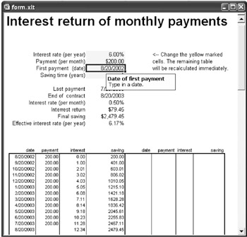
Figure 1-9: Interest on monthly deposits

From this input Excel calculates the date of the last deposit, the date the account terminates, the monthly interest, the crediting of interest, and the final total savings. Furthermore, Excel generates a table with monthly accrual of interest and balance, so that one can easily determine the balance at any time during the saving time.

The table can be used, for example, by a bank as the basis (and as promotional material) for convincing prospective customers of the value of opening a savings account. Creating a table tailored to the profile of a given customer can be accomplished in seconds. Finally, the table can be displayed in a suitable format.

Note	This example can be managed without macro programming, instead of being based on rather complex IF expressions. If you have difficulties with IF expressions, then see the information in the first section of Chapter 9.

The Model for the Table of Interest

The table is set up with a four-celled input region in which for simplicity of orientation input values have already been placed:

E5 (annual rate of interest): 6%
E6 (amount of each deposit): $100
E7 (first payment date): = Today()
E8 (time of savings): 1 year

From these data three results will be computed: the date of the last deposit ( n years minus 1 month after the first deposit), the end of the savings time (1 month thereafter), and the monthly rate of interest.

The determination of the date demonstrates the use of the Date function, by which a valid date is created from the data (year, month, day). The Date function is quite flexible: Date(1997, 13, 1) results 1/1/1998, Date(1998, 2, 31) in 3/3/1998, Date(1998, -3, -3) in 8/28/1997. It can be used almost without thinking; invalid month and day inputs are automatically translated into meaningful ones. The monthly rate of interest is simply one-twelfth of the annual rate (which yields an effective rate of “1 + (1 + 0.06/12)^12 = 0.06168, or 6.168%).

E10 (last deposit): =Date(Year(E7)+E8, Month(E7) ˆ’ 1, Day(E7))
E11 (end of account): =Date(Year(E7)+E8, Month(E7), Day(E7))
E12 (monthly interest rate): = E5/12
E15 (effective annual interest rate): = (1+E12)^12 ˆ’ 1

The actual results of the table ”the amount of interest credited to the account and the final balance ”result from the monthly table in the bottom area of the form (B17:I53). The crediting of interest comes from the sum of all the monthly interest payments, while the final balance is derived from the largest entry to be found in the two balance columns . (Since the length of the table depends on the length of time the account runs, there is no predetermined cell in which the result lies).

E13 (total of interest payments): = SUM(D17:D53, H17:H53)
E14 (final balance): =MAX(E17:E53, I17:I53)

We proceed now to the monthly table, whose construction involves the greatest difficulties with formulas. For reasons of space the table is conceived as having two columns. Thus the whole table, up to a savings time of six years, can be printed on a single sheet of paper.

The first row of the table is trivial and refers simply to the corresponding cells of the input region. In the interest column the initial value is 0, since at the time of the first deposit no interest has been credited.

B17 (date): = E7
C17 (deposit): = E6
D17 (interest): 0
E17 (balance): = C17

With the second row the general formulas begin, which after once being entered by typing in or copying are distributed to the entire table. Of significance here is that while formulas appear in every cell of the table, they should be shown only in a certain number of cells determined by the length of time the account runs. In the remaining cells the formulas must know that the savings time has been exceeded, and therefore give as a result an empty character string "" .

In the date column is tested whether the cell above contains a date (that is, is not empty) and whether this date is earlier than the date of account termination. If that is the case, then the new date is calculated by adding one month. In the deposit column is tested whether there is a date in the date column of the previous month . If that is the case, then the monthly deposit amount is shown, while otherwise the result is "" . The previous month test is therefore necessary, because in the last row of the table (account termination) there are no further deposits, but a final crediting of interest.

The date test occurs in the interest column as well. The formula returns the previous month's balance multiplied by the monthly interest rate, or else "" . In the balance column are added the previous month's interest and the deposit of the current month.

B18 (date): =IF(AND(B17<>"", B17<$E$11),
DATE(YEAR(B17), MONTH(B17)+1, DAY(B17)), "")
C18 (deposit): = IF(B19<>"", C17, "")
D18 (interest): = IF(B18<>"", E17*$E$12, "")
E18 (balance): =IF(B18<>"", SUM(E17, C18:D18), "")

Note that during formula input some of the cell references ($E$11, $E$12) are absolute. Otherwise, there will be problems in copying or filling in cells.

The formulas given for one row can now be copied downwards by filling in. Select the four cells B18:E18 and drag the small fill handle (lower right corner of the cell region) down to cell E53.

Excel's fill-in function is not capable on its own of adapting the formulas in such a way that the table will be continued in the second column. However, you can give it a bit of help by filling in the formulas of the first column for two more cells (to E55) and then shifting the region B54:E5 to F17 (select the cells and drag on the selection boundary with the mouse). Finally, you can fill in the second column with formulas just as you did the first.

Note

The formula for the date (B18) is in one respect not optimal:When 1/31/94 is given as start date, then the next date given is 3/3/94 (since there is no 2/31/94). Thereafter, all days of deposit are shifted by three days, the end date fails to agree with E11, and so on. This problem can be avoided if a new column is introduced containing a sequence of numbers for the deposits (1 for the first deposit, 2 for the second, etc.). Then the date of deposit can be calculated in the form DATE( YEAR(E7); MONTH(E7)+counter-1; DAY(E7)) .

Table Layout, Cell Protection, Printing Options

With the development of the formulas we have accomplished the most difficult task in our project. Now the table must be formatted in such a way that it presents a pleasing appearance (small, 8-point, type for the table of months, border lines, number and date formatting, alignment, background color for the input field, for example). With ToolsOptionsView you can deactivate the display of gridlines, row and column headers, horizontal scroll bar, and sheet tabs.

Now execute FilePrint Preview to see whether the table fits well on the page. If necessary you can adjust the height and width of individual rows and columns to obtain a better use of the space on the page. With the Layout button (or the menu command FilePage Setup) you can adjust the headers and footers (best is to select "none") and under the Margins tab select vertical and horizontal centering on the page.

Next you should protect your table against accidental changes made by the user . To do this, first select the input region and for these cells deactivate the option "Locked" (pop-up menu Format CellsProtection). Then protect the entire table (with the exception of the cells just formatted) using ToolsProtectionProtect Sheet. In the dialog that appears do not give a password.

Validation Control

The four input cells have been protected against erroneous input. This was accomplished with DataValidation, where the desired data format, validation rules, short information text, and a text for an error message (in the case of invalid input) were formulated. The possibility of formulating validation rules has existed since Excel 97.

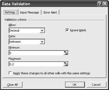
Figure 1-10: Formulation of validation rules for the interest table Templates

Templates

The table has now reached the stage where it can be used effortlessly: The user has merely to edit the four input areas and can then print out the result. To maintain the table in this condition and prevent it from being altered accidentally , save it with FileSave As in Template format in the directory Programs\Microsoft Office\ Office<n>\Xlstart (global) or Documents and Settings\username\Application Data\Microsoft\Templates ( user-specific ).

Templates are Excel files that serve as models for new tables. The user opens the template, changes certain information, and then saves the table under a new name. Excel makes sure automatically that the user gives a unique file name and does not overwrite the master template file with changes. In order for Excel to recognize templates, they must be saved in a particular format (filename *.xlt ) and in a particular place (see the preceding example).

Note	To test fully the special features of templates you should copy the sample file Intro5.xlt into one of the two above-mentioned locations. Furthermore, you must open it with the menu command FileNew, not FileOpen! (That would open the master file to allow you to make changes to it.)

Note

Further examples of templates and "smart sheets" can be found in Chapter 9, which is devoted entirely to the programming and application of such spreadsheets. For example, it is possible to write program code by means of which such tasks as automatically initializing the template on opening and providing buttons for printing are accomplished.