Section 9.1. Goal Seek

9.1. Goal Seek

I need $100,000. The bad news is that I only have $65,000. The good news is that I don't need the $100,000 until 60 months from now. So, I will put the $65,000 in the bank at 3.5% interest, and each month I will pay an amount into the account that will make it worth $100,000 after 60 months.

How much do I have to put in each month? The money in the account is earning interest, so the solution is not obvious. First, I build the worksheet in Figure 9-1.

Figure 9-1. Future value worksheet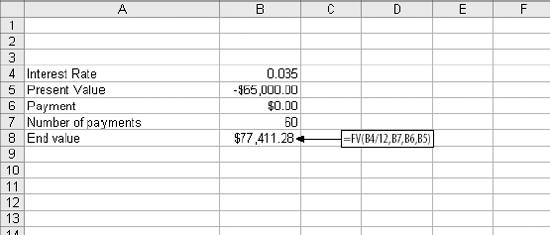

This models the problem. The interest rate is 3.5%. Present value is the amount I put in the account to start. It is negative because I am putting money in. The payment is zero for now. The number of monthly payments is 60.

The formula in cell B8 calculates the future value of the account. The formula is:

 =FV(B4/12,B7,B6,B5)

The 3.5% interest rate is per year. The FV function requires the interest per payment period (month in this case), therefore we divide by 12. The rest of the parameters, number of payments, payment amount, and starting value are values on the sheet.

This function returns a value of $77,411.28. This is how much the account will be worth if I make no monthly payment and rely totally on interest.

With the model built, we go to Tools Goal Seek and fill out the dialog as shown in Figure 9-2.

Figure 9-2. Using the Goal Seek tool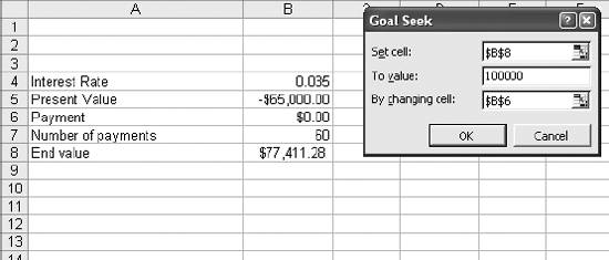

"Set cell" is the target cell. I want this cell to have a value of 100,000, so that's what I enter in the "To value" text box. "By changing cell" is the cell Goal Seek is allowed to change in order to reach the target value.

Click OK and Goal Seek finds the answer shown in Figure 9-3.

Figure 9-3. Goal Seek finds the payment amount

The payment in B6 is now -$345.04 and the End value is $100,000. So, it is going to cost me $345.04 for 60 months.

Goal Seek makes it easy to try different scenarios. If I can only afford a monthly payment of $275 how many more months will it take to get to $100,000?

The problem is set up in Figure 9-4.

Figure 9-4. Changing the problem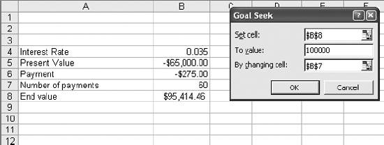

Here the payment is set at $275. Goal Seek has the same target cell and value, but is now allowed to change the number of payments in cell B7.

The result is in Figure 9-5.

It will take 68 months to reach the Goal with a $275 payment. (Actually, I will still be a few dollars short since it takes a little over 68 payments.)

Figure 9-5. The months needed to reach the Goal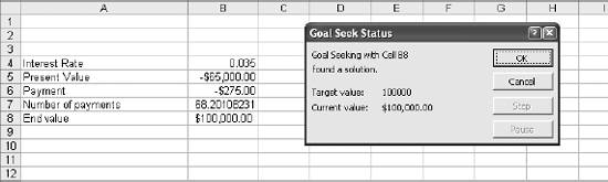

9.1.1. Setting a Price

Goal Seek can set the selling price of a product. Our customer wants to buy 1,200 units of a product we make. If we get the order, our fixed cost will be $1,500. Our variable cost is $52 per item. We want to set a price that gives a 20% profit.

We start by building the model in Figure 9-6.

Figure 9-6. The pricing model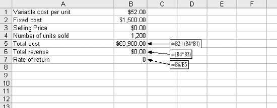

The selling price is zero for now, since Goal Seek will set it later. Total cost is the fixed cost plus the number of units multiplied by the variable cost.

Goal Seek is used as in Figure 9-7.

Our desired rate of return is fixed at 20% profit, so cell B7 is set to the target value of 1.2. Goal Seek is allowed to change the selling price in cell B3. The results are in Figure 9-8.

Our selling price is $63.90.

Figure 9-7. Goal Seek and the pricing model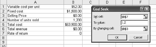

Figure 9-8. Results for the pricing model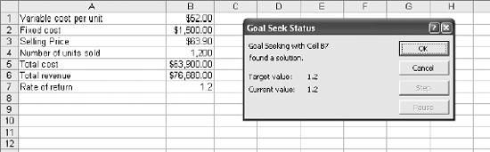

9.1.2. A Quadratic Equation

We can see a couple of Goal Seek's weaknesses when we use it to solve this quadratic equation:

 Y = X2 - .5X - 3

The problem is modeled in Figure 9-9.

The formula in cell B2 is the Excel equivalent of the equations, and it fills down to cell B8. The chart shows the relationship between X and Y. There are two solutions. They are the points where Y is zero. In the chart they are represented by the points where the Y plot crosses the x-axis. Figure 9-10 shows how the problem is set up.

The formula in column B is copied and pasted into cell B10. Cell A10 starts at 0. Goal Seek sets B10 to 0 by changing A10. The result is in Figure 9-11.

Goal Seek is not a perfectionist. It gets close and then quits. The real solution is, of course, -1.5. And there are two solutions to this equation. What about the other one? Goal Seek just finds a solution. If there are two or more possibilities it will not let you know.

Figure 9-9. A quadratic equation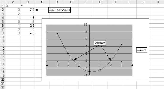

Figure 9-10. Setting up the quadratic problem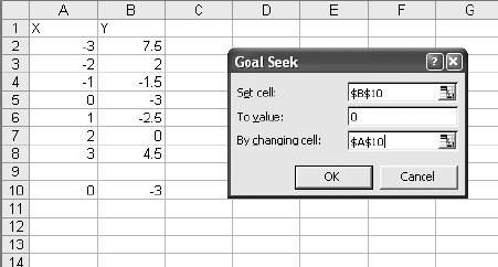

Which solution you get depends on what value you start with. In this case we started with 0 and -1.5 was the closest. If we had started with a value of 5, Goal Seek would have found the other solution, which is 2.

9.1.3. A Matrix Problem

The previous examples were simple, but Goal Seek can solve complex problems as well.

Suppose we work for a pharmaceutical company that makes a medication used by 1,000,000 people. We have a competitor that makes a similar medicine, and we each have half the market. It is easy for a customer to change medicines, and each month we keep 96% of our customers. The other 4% change to our competitor. But our competitor has the same problem, and each month they only keep 89% of their customers. We get the other 11%.

Figure 9-11. Goal Seek has found a solution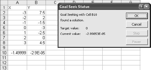

Today we have 50% of the market. If this situation continues for several months, our market share will stabilize at a new level. We need to figure out what our new market share will be.

Again we start by building a model, as shown in Figure 9-12.

Cells B2 and B3 contain the customer retention rates for our company and the competition. The matrix in Item 1 is based on these rates. In B5 and B6 are retention and loss rates or our company. In C5 and C6 are the same for the competition, but the order is reversed.

The vector in Item 2 represents the final market share. We start this at 1 to 1, as we do not know the ratio yet. This is the problem that Goal Seek will solve.

The matrix and vector are multiplied together using the MMULT function, which is an array formula that returns the product.

The ending ratio is a vector that does not change when multiplied by the matrix. So if the vector (cells B8 and C9) is equal to the product of the matrix and the vector (cells B11 and B12), then we have solved the problem. The test value is 0 when the problem is solved.

The rest of the sheet breaks down the customer population and calculates our ending market share.

We are not going to cover the theory behind the matrix calculation in this example. It uses an eigenvector , which is a value encountered in linear equations .

With the model built, we use Goal Seek to solve the problem as shown in Figure 9-13.

Figure 9-12. Modeling the problem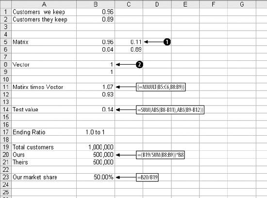

Here we want Goal Seek to set the test value in cell B14 to zero by changing B8. Only the top cell in the vector needs to change since we are looking for a ratio. Any ratio can be expressed as X/1.

The solution is in Figure 9-14.

The ending ratio will be 2.75 to 1, and our market share will increase from 50% to 73.33%.

9.1.4. Using Goal Seek in a Macro

Goal Seek can become part of an application. Suppose we need to calculate market share at different retention rates. We can add a macro to the worksheet that runs Goal Seek automatically.

When Goal Seek runs from a macro it does not display the ending dialog, so it requires no user interaction.

Figure 9-13. Using Goal Seek to solve the market share problem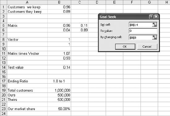

Figure 9-14. The solution to the market share problem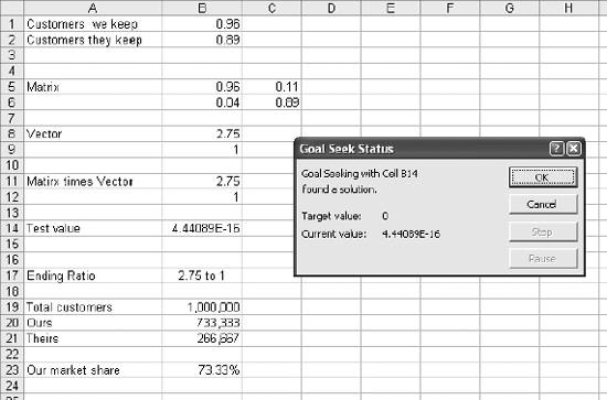

To add code to the sheet we go the Visual Basic Editor either by clicking Tools Macro Visual Basic Editor or by pressing Alt-F11.

Once the editor is running, the options shown in Figure 9-15 are selected.

Figure 9-15. Adding code to a worksheet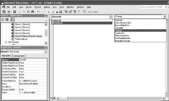

Most VB code is in a module, but in this case we put the code inside the worksheet. In Item 1 we select the sheet containing the market share problem.

In Item 2 we select the worksheet itself. This exposes the worksheet's events, and in Item 3 we select the Change event.

This puts an empty change event macro in the worksheet. A change event fires every time the user changes the contents of a cell on the worksheet. The following code is added to the change event macro:

 Private Sub Worksheet_Change(ByVal Target As Range) If Target.Column = 2 And Target.Row < 3 Then     Range("B14").GoalSeek Goal:=0, ChangingCell:=Range("B8") End If End Sub 

Excel passes a range object called Target to the macro. It contains information about the changed cell including column and row properties. The range object has an Address property, but since we are interested in two cells we use Column and Row to decide if the changed cell is B1 or B2. If it is, we run Goal Seek. If not, we don't.

The statement that runs Goal Seek answers the questions the Goal Seek dialog asks. We are still asking for cell B14 to be changed to zero by changing B8.

With this code in place the worksheet will update every time either retention rate changes.