Section 7.3. The Logic

7.3. The Logic

The application is designed simply. All the logic is on the Workarea sheet. It uses the usual conventions. The first section of this sheet is shown in Figure 7-6.

Figure 7-6. The first section of the Workarea sheet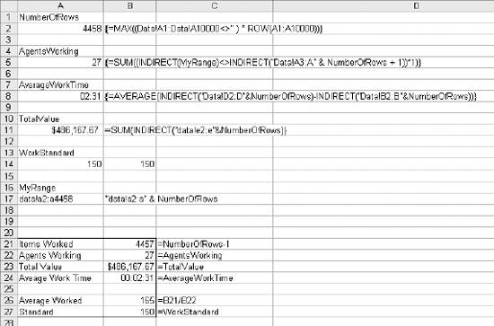

The application needs to be flexible. For 2/19/2004 we have 4457 rows, but the next day could be any number. So, we need to know how much data is on the Data sheet. To find the bottom row of the worksheet, we use this formula in cell A2:

 {=MAX((Data!A1:Data!A10000<>"" ) * ROW(A1:A10000))}

There are other ways to do this, but this formula lets us work with the column we need and keeps the calculation on the worksheet. This is an array formula and is entered by pressing Ctrl-Shift-Enter simultaneously. It looks at the rows from 1 to 10,000 and works by building two lists of values. The first list (Data!A1:Data!A10000<>"") is just 10,000 zeros or ones. The value is 1 for cells in the range that contain data and 0 for those that are empty.

The second list (ROW(A1:A10000) is the numbers from 1 to 10,000. The lists are multiplied together. Row numbers with data are multiplied by 1, while empty row numbers are multiplied by 0. The formula takes the maximum value from the products, which is the row number of the last row used.

The result of this formula is named NumberOfRows. This is a powerful formula and can be modified to find the last column used or the last row containing a specific value.

We will refer to column A (agent) on the Data sheet several times. To save keying, we build a reference to the range that contains the data. Cell A17, named MyRange, contains this formula:

 ="data!a2:a" & NumberOfRows

We can use MyRange in other formulas, such as the one in A5:

 {=SUM((INDIRECT(MyRange)<>INDIRECT("Data!A3:A" & NumberOfRows + 1))*1)}

We need to know how many agents are working. This is not the same every day, so it needs to be calculated. Again we use an array formula. We know the Data sheet is sorted by agent, and we count the times the agent changes. The formula builds a list of zeros and ones. It is 1 only for cells that are not equal to the cell on the next row.

We use indirect functions because we do not know how many rows there will be. The second INDIRECT points to a range that is one row lower than MyRange.

The time it takes to work an item is the completed time minus the assigned time. In cell A8 the formula is:

 {=AVERAGE(INDIRECT("Data!D2:D"&NumberOfRows)-INDIRECT("Data!B2:B"&NumberOfRows))}

The completed times are in column D of the Data sheet and the assigned times are in column B. This array formula takes the average of the work times. The result is named AverageWorkTime. We also want to know the total value of work done, so in cell A11 the formula is:

 =SUM(INDIRECT("data!e2:e"&NumberOfRows)

The work standard in cell A14 is entered as a number and can be changed as needed.

The range A21:B27 is named DailyTotals. It is a display area and appears on the Totals sheet, Figure 7-2, as Item 4. It is referenced as an array formula. The range B8:C14 on the Totals sheet contains the formula:

 {=DailyTotals}

Figure 7-7. Agent names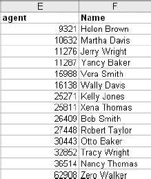

The Data sheet only has employee numbers, and we want to display the names as well. The table of employee numbers and names is in columns E and F of Workarea, as shown in Figure 7-7.

On the Totals sheet information is summarized by agent. The next part of Workarea contains the logic. The Data sheet is sorted by agent and assigned_date, making it easier to arrange the information by agent. This area is shown in Figure 7-8.

Figure 7-8. More Workarea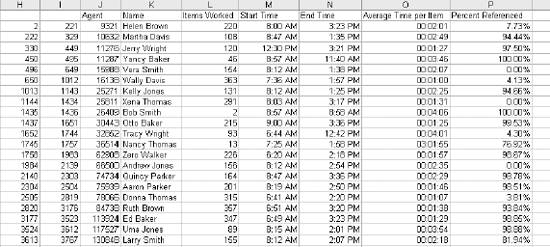

The first step is to determine the range of rows for each agent. This is done in columns H and I. The formula in column I finds the last row for each agent. It contains this formula:

 =MATCH(J2,INDIRECT(MyRange),1)+1

Cell J2 contains the agent number. MyRange is a named value equal to data!a2:a4458. Option one in the match function returns the row with the largest value less than or equal to J2. We add 1 because MyRange starts in row two. This formula fills down for 50 rows. If more than 50 agents could be working, additional rows can be used.

Cell H2 contains the number 2. The first row number of the first agent is always 2. Cell H3 is set to one more than cell I2, since the first row for each agent is one more than the last row for the agent above. This formula also fills down.

The first cell in the agent column (J2) is set equal to cell data!a2, since that is the first agent number. The formula in cell J3 is:

 =IF(ISERROR(INDEX(INDIRECT(MyRange),I2+1)),"",INDEX(INDIRECT(MyRange),I2+1))

This formula uses an INDEX function on MyRange. It points to the row after the last row for the agent above. The application will handle up to 50 agents but not all 50 are used in this example. After the last agent the INDEX function will generate an error. The IsError function is used to set the cells that are not used to blank.

Column K contains the agent name. The formula is:

 =IF(J2="","",LOOKUP(J2,Agent,Name))

The IF function checks to be sure the current row is used. If it is, the LOOKUP function finds the value J2 in the range named Agent. It returns the value from the range Name.

The items worked in column L is based on the number of rows and is calculated with this formula:

 =IF(J2="","",(I2-H2)+1)

The start and end times are on the first and last rows for the agent. For the start time we use the assigned_date (column B) since that is when the agents got their first piece of work for the day. For the end time we use completed_date (column D). The formulas are:

 =IF(J2="","",INDIRECT("data!B" & Workarea!H2)) =IF(K2="","",INDIRECT("data!D" & Workarea!I2)) 

Average time per item is calculated using:

 {=IF(J2="","",AVERAGE(INDIRECT("data!d" & H2 & ":d" & I2)-INDIRECT("data!b" & H2 & ":b" & I2)))}

This takes the average of the difference between the completed and assigned times for the agent. It is an array formula. The values H2 and I2 in the INDIRECT functions are the starting and ending rows for the agent.

To get the percent of items referenced we count the number of cells in column C that are not empty and divide by the number of rows for the agent. The formula is:

 =IF(J2="","",(COUNTIF(INDIRECT("data!c" & H2 & ":c" & I2),">0"))/L2)

This gives us a display area for the Totals sheet. But we are giving the user the ability to sort this information. This is complicated because all the information is linked and we cannot use Excel's sort tool directly.

7.3.1. Using a Tag Sort on Linked Information

We use a tag sort to get around this problem. A tag sort uses pointers to control the display order of the rows. We use the sort tool to sort the tags rather than the data. The tag sort area is shown in Figure 7-9.

Figure 7-9. The tag sort area of the Workarea sheet

Column R contains row numbers. These are just the numbers from 1 to 50 and correspond to the row numbers in the range J2:P51. These row numbers control the order of the same information in the range U2:AA51.

The formula in cell U2 is:

 =INDEX(J$2:J$51,$R2)

This formula points to column J. The rows in the range are locked with $. The index is in R2 and its column is locked. This formula is filled right and down for the whole range U2:AA51.

As a result, columns U:AA look exactly like columns J:P. But if the order of the numbers in column R changes, the order of the rows in U:AA will also change. The range U1:AA51 is named AgentList and is displayed on the Totals sheet using the array formula:

 {=AgentList}

When the user clicks on one of the headings, the tag sort is performed. It is a two step procedure. Sorting by Items Worked, the tag sort area is shown in Figure 7-10.

Figure 7-10. Tag sort on Items Worked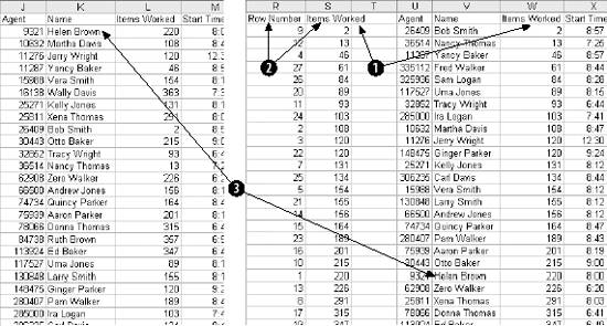

In Item 1 the information in column W (Items Worked) is copied and pasted (Paste Special Values) into column S.

Next, in Item 2, columns R and S are sorted ascending on column S.

Item 3 shows the result, in which the first agent (Helen Brown) is now on the 22nd row of the AgentList range. The Totals sheet only sees this range, so the display is now sorted.

This is done with two macros. The first contains only one line. If the user clicks on Items Worked, the sort needs to be on column W. A macro named Sortw runs, passing the value w to a function named Sortit. Here is the code:

 Sub Sortw(  ) R_code = Sortit("w") End Sub 

Sortit is a custom function written for this application. It can sort AgentList for any column. It gets the column as a passed value. This is the Sortit macro:

 Function Sortit(MyCol As String)     Dim ToSort As String     'Turn off screen updating so the user will not     'see all of the steps     Application.ScreenUpdating = False     'MyCol contains the column to be sorted. It is a value from U to AA     'depending on which column the user selected.     'MyRange holds the range of cells to be sorted. Agentsworking     'is a named value on workarea and contains the number of     'agents working. We add one to include the heading.     MyRange = MyCol & "1:" & MyCol & Range("agentsworking").Value + 1     'The sort is performed on the workarea sheet     Sheets("Workarea").Select     'Copy the cell range to be sorted     Range(MyRange).Copy     'Move to the S column     Range("S1").Select     'Perform a PasteSpecial Values     Selection.PasteSpecial Paste:=xlPasteValues, Operation:=xlNone, SkipBlanks _         :=False, Transpose:=False     'ToSort holds the range to be sorted.     ToSort = "r1:s" & Range("agentsworking").Value + 1     'Select the sort range     Range(ToSort).Select     'Perform the sort     Selection.Sort Key1:=Range("S2"), Order1:=xlAscending, Header:=xlGuess, _     OrderCustom:=1, MatchCase:=False, Orientation:=xlTopToBottom, _     DataOption1:=xlSortNormal     'Return to the Totals sheet     Sheets("Totals").Select     'Turn screen updating back on     Application.ScreenUpdating = True End Function 

The Sortw macro runs when the user clicks on the Items Worked heading on the Totals sheet.

7.3.2. Invisible Rectangles

This happens because there is a rectangle object over the heading. The setup is shown in Figure 7-11.

If the drawing toolbar is not visible, you need to go to the View Toolbars menu and check Drawing. A rectangle is drawn over the heading. Then right-click on the rectangle and select Format AutoShape. The dialog in Figure 7-12 will display.

The rectangle has no fill and no line making it invisible. Next we assign the Sortw macro to the rectangle. We right-click again and select Assign Macro. This brings up the dialog in Figure 7-13.

The rectangle is invisible but still responds to the click event.

Figure 7-11. Adding a rectangle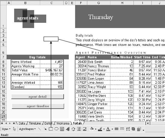

There is a separate macro (Sortu, Sortv, .... etc) for each column and a separate rectangle for each heading.

7.3.3. The Agent Detail Area

On the Detail sheet the user can select an agent. When this happens, Workarea needs to calculate metrics for the agent, populate the chart, and build the timeline.

Totals for the selected agent are calculated in the range shown in Figure 7-14.

Cell A40, named AgentRow, is linked to the listbox on the Detail sheet. The value tells which agent the user selected. The value in cell A42 gives the starting row for the agent. This is the row on the Data sheet that starts this agent's information. This value is in the H column at the row given by AgentRow. The cell is named AgentStartRow and the formula is:

 =INDEX(H2:H51,AgentRow)

AgentEndRow works the same, getting its value from column I with the formula:

 =INDEX(I2:I51,AgentRow)

Figure 7-12. Making the rectangle invisible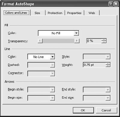

Figure 7-13. Assigning the macro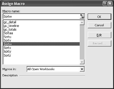

The number of items worked is the number of rows. The formula in cell A46 is:

 =AgentEndRow-AgentStartRow

Figure 7-14. Agent totals on the Workarea sheet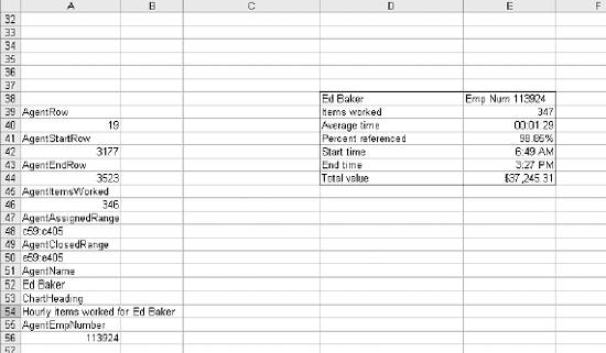

This returns a value one less that the number of rows because the first row is not zero. This situation comes up all the time when working with cell ranges. We need this value for more than one thing. For building ranges this is fine, but when we display the number of items worked we will add 1 to the value.

The ranges for the assigned_date and completed_date are used in other calculations. So, to simplify things we will build the ranges and name them. The formulas are:

 ="c59:c" & 59+AgentItemsWorked ="e59:e" & 59+AgentItemsWorked 

AgentName, cell A52, is from column K and uses this formula:

 =INDEX(K2:K51,AgentRow)

The chart heading is just text and uses AgentName. The cell (A54) is not named because names cannot be used in chart headings. The formula is:

 ="Hourly items worked for " & AgentName

AgentEmpNumber is extracted from the J column with this formula:

 =INDEX(J2:J51,AgentRow)

The range D38:E44 is named AgentDetail. It is displayed on the Detail sheet as an array. The relationship is shown in Figure 7-15.

Using this technique keeps the display and the logic separate.

Figure 7-15. Using an array formula to display a named range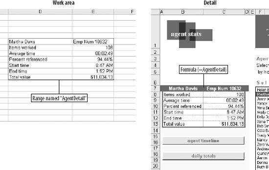

7.3.4. The Chart Area

The chart on the Detail sheet is populated using the range J58:M82. This range is not named, and is shown in Figure 7-16.

The numbers in column J are the hours of the day. The same hours are displayed using a time format in column K. The numbers in column J are used by the array formula in column L:

 {=SUM((HOUR(INDIRECT(AgentAssignedRange))=J59)*1)}

The formula checks the range containing the assigned dates and counts the number that are in each hour. It fills down for all the hours.

Column M is the standard. Each day an agent is expected to work 150 items. This is in the cell named WorkStandard (A14). A workday has seven hours. So, column M contains the integer value of 150/7. It is the number of items an agent must work each hour to meet the goal.

The range K58:M82 is selected and the chart is added by selecting Insert Chart from the menu. This is a Line - Column chart found on the Custom Types list, as shown in Figure 7-17.

The chart is placed on the Detail sheet using the dialog in Figure 7-18.

Figure 7-16. The chart on the Detail sheet uses this area

It results in the chart shown in Figure 7-19. This is the basic chart for the application. It can be positioned and sized by dragging. It will be further customized on the Detail sheet.

The first step is to remove the markers on the standard line and change the color and weight of the line. We start by right-clicking on the standard line (Item 1 in Figure 7-19). We select Format Data Series and the dialog in Figure 7-20 displays.

We click on the Patterns tab and set the options as shown in Figure 7-20. The bars showing the hourly counts need to be changed to blue. The process is the same as for the standard line. We right-click on the count bar (Item 2 in Figure 7-19) and change the Patterns tab.

Next, we change the alignment on the X axis . The times are displayed diagonally and are hard to read. So, right-click on the axis (Item 3 in Figure 7-19) and select the Alignment tab. The orientation is set as shown in Figure 7-21.

Finally we link the chart title to cell A54 on Workarea, but the chart tool won't let us do this directly. So, we start by adding a simple title that can be edited. With the chart selected, we select Chart Chart Options from the menu. This displays the dialog shown in Figure 7-22.

Figure 7-17. Inserting the chart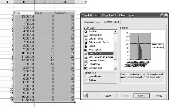

Figure 7-18. Putting the chart on the Detail sheet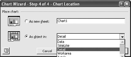

We enter a title of XXX to make it easy to edit. After the title is on the chart, we right-click on it. Then the formula is entered in the formula bar, as shown in Figure 7-23.

This links the title to the Workarea sheet and when the user selects a new agent the title will change along with the chart.

Figure 7-19. The basic chart ready to be customized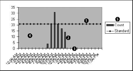

Figure 7-20. Formatting the standard line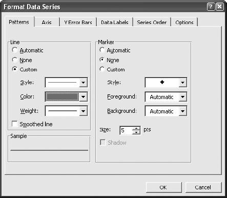

7.3.5. The Timeline

The last area in the Workarea sheet is the display range for the timeline. We are allowing for 500 items for an agent in one day. In this application that will be enough, but if more are needed it is simple to fill the formulas down further and increase the size of the named range. Figure 7-24 shows the range.

Figure 7-21. Setting the alignment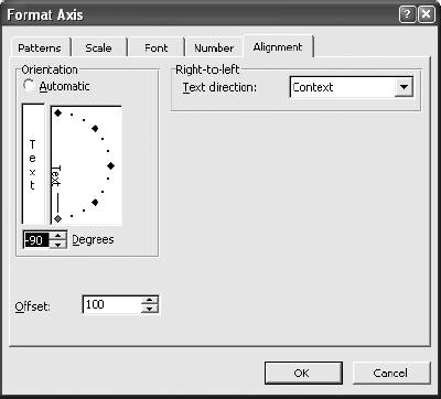

Figure 7-22. Adding a chart title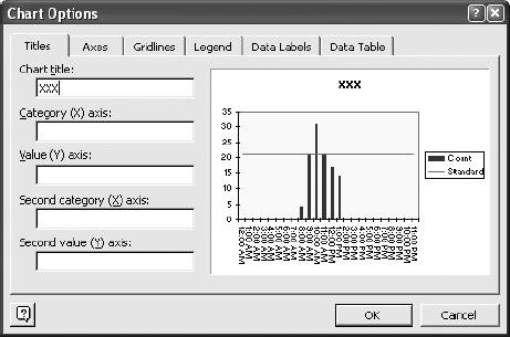

Column A contains row numbers on the Data sheet. They give the location of the agent's data. It is not part of the display and is used to map the agent's rows on the Data sheet to this part of the Workarea sheet. The first cell (A59) is set equal to the named value AgentStartRow. Cell A60 contains this formula:

 =IF(A59<AgentEndRow,A59+1,"")

Figure 7-23. Customizing the chart title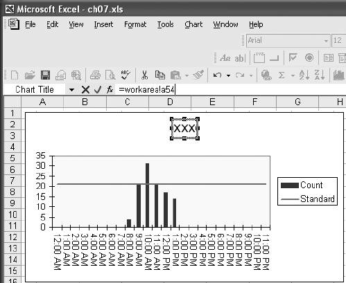

Figure 7-24. The display area for the Timeline sheet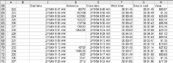

This formula fills down and gives us the row numbers of the data we need.

Columns C, D, E, and H all use the same basic formula. Cell C59 contains:

 =IF($A59="","",INDIRECT("data!" & ADDRESS($A59,COLUMN(B1))))

The IF function checks to see if we have reached the end of the agent's data, and if so it returns a blank. The ADDRESS function takes a row and column and returns an address. In this case ADDRESS($A59,COLUMN(B1)) is equivalent to ADDRESS(222,2) and returns a value of $B$222. We combine this with the sheet name (Data is the sheet we are referencing) and use the resulting reference in an INDIRECT function. This returns the first assigned_date for the agent. This formula fills down and across, covering columns C, D, E, and H.

Work time and "Time to next" are calculated as in other parts of the application by using these formulas:

 =IF(A59="","",E59-C59) =IF(A60="","",C60-C59) 

On the Timeline sheet this area is referenced by the name TimeLine.

7.3.6. Navigation

The navigation buttons are from the Forms toolbar. They are formatted to use a font color that matches the color scheme of the application and they are each assigned a macro. There are three macros, one for each display sheet. They each have only one line, and this is the code:

 Sub go_detail(  ) Sheets("detail").Select End Sub Sub go_totals(  ) Sheets("totals").Select End Sub Sub go_timeline(  ) Sheets("timeline").Select End Sub 

This code provides simple navigation. The user clicks the button and the destination sheet is selected.