Section 1.3. Statistical Functions

1.3. Statistical Functions

Statistical functions are used to describe data. When working with a list of numbers, we need to be able to find the average, to understand any trends, and to describe the distribution. In this section we look at Excel's most commonly used statistical functions .

1.3.1. The Average

The average is the most common measure of the center of a group of numbers, and Excel makes taking an average easy. The basic approach is shown in Figure 1-6.

Figure 1-6. Taking an average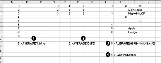

Five is the average of the numbers from one to nine (in column A, rows 1 through 9). Usually numbers will be in a column, as in item 1, but it really doesn't make any difference as long as you know where the numbers are. In item 2 the average formula is looking at a three by three range, and in item 3 the numbers are mixed with non-numeric information.

Excel ignores cells that do not contain valid numbers, and item 4 uses this behavior to simplify taking the average of scattered numbers. The AVERAGE function finds the numbers in the range. I don't have to tell Excel where they are.

1.3.1.1. AVERAGEA

The AVERAGE function is usually convenient, but fails in Figure 1-7.

Figure 1-7. Averaging text as a number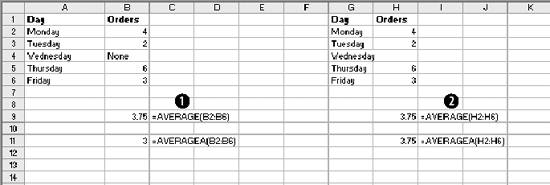

On Wednesday we did not get any orders. The data contains the word "None," but the value is really zero. In item 1, the AVERAGE function gets the wrong answer because it ignores the cell with "None" in it. The AVERAGEA function is made for this situation. AVERAGEA works just like AVERAGE, except it considers non-numeric cells to have a value of zero. In item 1 formula 2, the AVERAGEA function calculates the average correctly.

AVERAGEA ignores cells that are not used. In item 2, the Orders cell for Wednesday is empty and the AVERAGEA function does not consider the cell to have a value of zero.

1.3.1.2. DAVERAGE

Excel can also calculate the average of selected items in a list using the DAVERAGE function. Figure 1-8 shows how this function is used.

Figure 1-8. Using DAVERAGE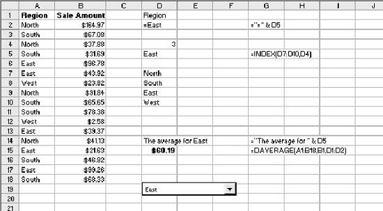

The range A1:B18 contains sales amounts and regions. This worksheet allows the user to get the average of a selected region.

First we give the user a way to choose a region. We enter the region names in D7:D10. Then we add a combo box using the forms tool bar shown in Figure 1-9.

Figure 1-9. Adding a combo box

If the forms tool bar is not visible, go to the View Toolbars menu and check Forms.

We click on the combo box icon and drag it to the sheet. Then we right click on it and select Format Control. This displays the dialog in Figure 1-10.

Figure 1-10. Formatting the combo box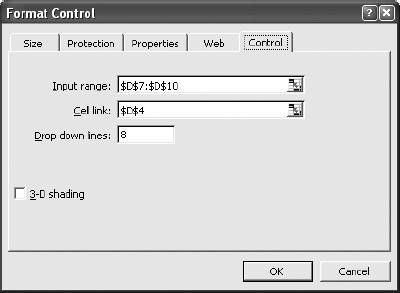

The Input range tells the combo box what values to display. The region names are in the range D7:D10, so that is the Input range.

The Cell link is D4. When the user selects one of the four regions, the combo box puts a number in the Cell link telling which region was selected. The Cell link does not get the region name, only a number. In Figure 1-8, East is selected. East is the third item in the list of regions, therefore the Cell link (D4) contains the number three.

We need the name of the selected region, and to get it we use the formula in cell D5 in Figure 1-8:

 =INDEX(D7:D10,D4)

The INDEX function returns an item from a range. The range D7:D10 contains our region names. Cell D4 has the number three. The INDEX function returns the third item in the range, the name "East".

The DAVERAGE function is in cell D15 and has this formula:

 =DAVERAGE(A1:B18,B1,D1:D2)

There are three parameters. The first is the range A1:B18, containing all of the data including column headings. Next is B1. This is the heading of the column we want to average. The formula could have been entered as:

 =DAVERAGE(A1:B18,"Sales Amount",D1:D2)

The third parameter is the criteria range. It consists of a heading and a logical test. The heading tells the function what column to apply the test to. DAVERAGE takes the average of the rows where the test is true.

We are only averaging sales amounts for East. The criteria range is D1:D2. The formula in D2 is:

 ="=" & D5

This uses the result of the combo box selection in cell D5 and builds the text string "=East".

This makes the sheet interactive without using a macro. The DAVERAGE function in cell D15 calculates the average for the selected region as soon as the user changes the selection.

DAVERAGE is a database function. Database functions allow you to perform common calculations on worksheet data. But the data has to be set up correctly for them to work. They require headings and a criteria range. This is fine if you are designing an Excel solution from scratch, but can lead to complications if you are adding calculations to an existing sheet.

Excel has a wide range of functions, and in most situations there is more than one way to get the desired result. In this case, I could replace the DAVERAGE function in cell D15 with this formula:

  =SUMIF(A2:A18,D2,B2:B18)/COUNTIF(A2:A18,D2)

It uses the SUMIF and COUNTIF functions to get the same answer, avoiding the formatting requirements of database functions . There is no best way to do this. It depends on how the sheet is designed and what you are trying to accomplish.

1.3.1.3. Trimmed average

All numbers are not created equal. In examples, like the ones in this chapter, the numbers are made up. They can't be wrong because they don't mean anything. In the real world things are different.

Numbers can be recorded incorrectly, unusual events can produce odd values that confuse our view of the past and make the average inaccurate. These troublesome values are called outliers or anomalies .

When we use data that might have outliers we can increase the accuracy of calculations by ignoring the highest and lowest values. This is also sometimes called a filtered average. Excel does this with the TRIMMEAN function.

In Figure 1-11 you can see how this works.

Figure 1-11. A trimmed average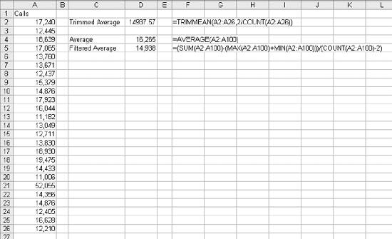

We want the average number of calls per day handled by a call center. Figure 1-11 has the call count for the 25 most recent days. But in cell A21 something is wrong. A network problem on that day incorrectly routed tens of thousands of calls to our call center.

If we just take the average we get 16,265. But that is not good estimate of the real average, since it includes the problem data. We can get a better estimate by using this formula:

 =TRIMMEAN(A2:A26,2/COUNT(A2:A26))

The first entry in the trIMMEAN function is the range of cells to be averaged. The second entry is the percentage of cells to ignore. In this case I want to eliminate the maximum and the minimum values. Therefore, I need to set the value to trim only one item at the top and bottom of the distribution. That is equal to two divided by the number of items.

This is equivalent to this formula:

 =(SUM(A2:A100)-(MAX(A2:A100)+MIN(A2:A100)))/(COUNT(A2:A100)-2)

This takes the sum of all the numbers, subtracts the maximum and minimum, and then divides by two less than the item count.

It would be nice to have a function that just removes the maximum and minimum, and a custom function can do just that.

First we go to the Tools Macros menu and select Visual Basic Editor. The editor can also be started by pressing Alt-F11. This code is then entered:

 Public Function FAverage(MyRange As Excel.Range) As Double 'Find the sum of the range FAverage = Application.WorksheetFunction.Sum(MyRange) 'Subtract the maximum value FAverage = FAverage - Application.WorksheetFunction.Max(MyRange) 'Subtract the minimum value FAverage = FAverage - Application.WorksheetFunction.Min(MyRange) 'Divide by two less than the count of values in the range FAverage = FAverage / (Application.WorksheetFunction.Count(MyRange) - 2) End Function 

We do not have to actually code the logic to calculate the sum, maximum, or minimum, because the application object already knows how to do these things. In effect, we are using normal Excel functions inside our code. With this code in place, our sheet has a new function called FAverage. Its only parameter is the range of cells we are working with, and it returns the filtered average.

A custom function is fine for a one-off problem, but you may want to reuse your solution later, or there may be other Excel users doing a similar job who could use the same function. If this is the case, an Excel Add-In is an easy way to publish one or more custom functions.

We start with a new blank workbook. We bring up the Visual Basic Editor as before and add the same code. We save the workbook with the name StatHelper as an Excel Add-In. It will be saved with an extension of .xla in your Application Data/Microsoft/AddIns folder.

Then exit and restart Excel, and bring up another blank workbook. Go to the Tools Add-Ins menu and you will see StatHelper on the list of available Add-Ins. Make sure it is checked, and your new workbook will have the FAverage function.

You can distribute the StatHelp.xla file to others. It needs to be placed in their Application Data/Microsoft/AddIns folder. You can add additional functions to your XLA file, or even make it a group project with functions added by other users.

1.3.1.4. Moving average

Tracking changes in the average is an easy way to find trends in data. A moving average is shown in Figure 1-12.

Figure 1-12. The moving average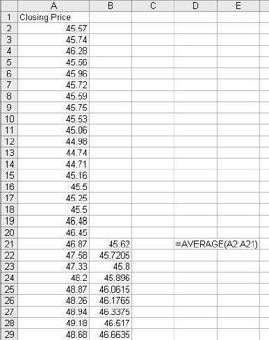

In this example we have 65 days of closing prices for a stock. The formula in cell B21 takes the average of the preceding 20 days. The formula fills down, creating a moving average.

Moving averages are often used in charts to make trends easy to understand.

1.3.2. Changes in the Average

The simplest change is a linear trend. In business this means the value is going up or down by the same amount each time period (e.g., each month sales are going up by $10,000). The TREND function can identify the points on the trend line or forecast future values. Figure 1-13 shows how the trEND function can build a trend line.

Figure 1-13. Finding the trend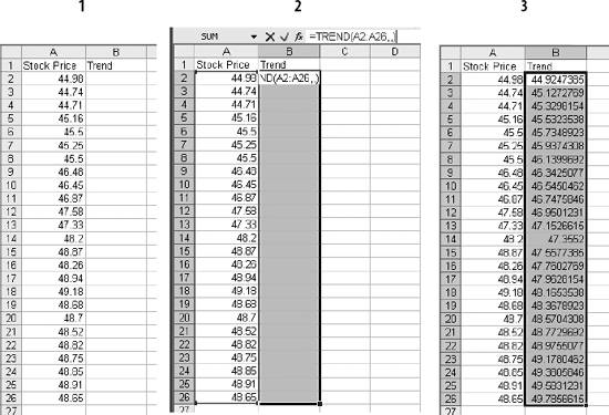

In Step 1 are the closing stock prices for 25 days. In column B is a heading for the trend.

In Step 2, we select the range B2:B26 and click on the formula bar. In the formula bar we enter the following:

 =TREND(A2:A26,,)

The trEND function has three parameters. First is the range of the Y values. In this case these are the stock prices. The next parameter is the range of the X values. When we are working with a value that is changing over time, like a stock price, these are just the numbers 1,2,3...to the number of values, 25 in this case. This is the default, so we don't have to enter anything except a comma as a place holder. The third parameter is the X values we want the function to return. Here we also take the default. This is an array formula and must be entered with Ctrl-Shift-Enter. The result is shown in Step 3.

The result is a line. Each value in column B goes up by the same amount, in this case by 0.202538. If we build a chart using the data in columns A and B, it will look like Figure 1-14.

The TREND function can also forecast future values . The next value can be predicted with this formula:

 =TREND(A2:A26,,COUNT(A2:A26)+1)

Figure 1-14. Chart with trend line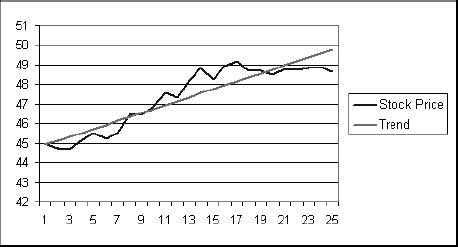

The COUNT function returns the number of cells in the range. Adding one tells the trEND function that we want the next value.

Forecasting the next value is something that we might want to do from time to time, and it would be convenient if we had a function to do this based only on the range.

We can create a custom function with this code:

 Public Function TrendNext(MyRange As Excel.Range) As Variant 'Find the next value from a range using the TREND function TrendNext = Application.WorksheetFunction.Trend(MyRange, , _ Application.WorksheetFunction.Count(MyRange) + 1) End Function 

Once again, we use the application object to get to Excel's built-in functions. If this code is added to the StatHelper.xla, the TRendNext function will be ready to use. Figure 1-15 shows an example.

Figure 1-15. Using the TrendNext function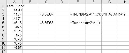

Both formulas return the same value, but TRendNext is specialized and easier to use.

1.3.2.1. Growth

Trends are not always linear. Values can go up or down in ways that cannot be described with a line. Exponential growth is based on multiplication. In a linear trend each item changes by the same amount. In growth each item changes by the same ratio. Excel has a GROWTH function that models exponential growth . It works just like the TREND function but returns different results.

Figure 1-16 demonstrates the difference between the GROWTH and TREND functions.

Figure 1-16. GROWTH and TREND measure different things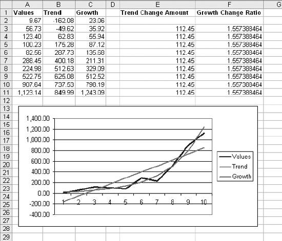

Here the values in column A are changing exponentially. We use both the GROWTH and trEND functions to try to model the values. In the chart it is clear that the GROWTH function does a better job. The trend line doesn't really explain what the values are doing, and even starts with a negative value.

If we predict the next few values in this series, we will get better results if we use GROWTH.

Column E shows how the trEND function works. It starts with -162.08 and adds 112.45 each time. This gives the best fitting line possible for the values. In Column F the GROWTH function starts with 23.06 and multiplies by 1.557 each time. This produces the best fitting exponential curve.

In most business situations the trEND function works fine. But GROWTH makes more sense when working with returns on investments, inflation rates, or other values that change by a percentage over time.

It is easy to see how the data is behaving in these examples, but in the real world trends are likely to be subtle and the data less consistent. It is important to understand the data before you choose which function to use. It is helpful to look at a chart before deciding between GROWTH and TREND.

1.3.3. Distributions

The average number of calls coming into a call center is 12,534 per day. But a day with exactly 12,534 is rare. If we are going to manage this process, we need to know how spread out the data is and how it is distributed.

Excel offers functions to handle the kinds of distribution most frequently encountered in business.

1.3.3.1. Normal distributions

A normal distribution has a bell shaped curve. Most of the values are near the middle. The tails of the distribution contain uncommonly high or low values. This is the most common distribution in business situations.

The simplest measure of a normal distribution is the variance . To calculate the variance, each value is subtracted from the average and the difference is squared. Then the squared differences are summed and the sum is divided by one less than the number of values. In Excel all this is done by the VAR function. Figure 1-17 shows how this works.

We will calculate the variance of the 20 numbers in column N. The formula in cell O1 is:

 =(N1-AVERAGE(N$1:N$20))^2

It takes the difference between the value in cell N1 and the average of all 20 cells. This fills down to row 20.

Cell Q6 contains this formula:

 =SUM(O1:O20)/19

Figure 1-17. Calculating the variance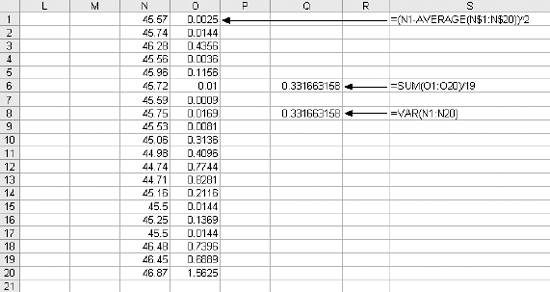

It sums the squared differences and divides by 19 (one less than the number of values).

In cell Q8 we let Excel do the work by using the VAR function and get the same result.

The most commonly used measure of spread is the standard deviation. Standard deviation is just the square root of the variance, and Excel has the STDEV function to calculate it.

The standard deviation is used in many statistical calculations. Once you have the average and the standard deviation, Excel has functions that can tell you how a value fits into the distribution. This is illustrated in Figure 1-18.

We want to know where 46.75 fits in the distribution, and we know the average and standard deviation. The NORMDIST function gives us the answer. In Figure 1-17 cell Q1 has the average and Q2 has the standard deviation. The formula is:

 =NORMDIST(46.75,Q1,Q2,TRUE)

The first entry is the value we want to test (46.75). Next are the average and standard deviation. Finally, we use the option trUE to get the cumulative probability for 46.75. If we entered FALSE for this option, the function would return the height of the distribution curve at 46.75.

The NORMDIST function returns a value of 0.9751. This means that 97.51% of the distribution is below 46.75.

The NORMINV function works in the opposite direction. Suppose we need to know what values are in the top 25% of the distribution. The value we need is the one at the 75% point. For the data in Figure 1-17 this formula will find the answer:

 =NORMINV(0.75,Q1,Q2)

Figure 1-18. Using the average and standard deviation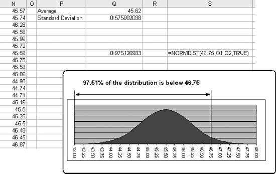

The first entry is the percentage we are looking for. Next are the average and standard deviation. This function has no TRUE/FALSE option. The formula returns a value of 46. The values 46 and above are the top 25% of the distribution.

1.3.3.2. Exponential distributions

Our call center gets three calls every ten minutes. The time between calls has a distribution illustrated in Figure 1-19.

Figure 1-19. Distribution of call times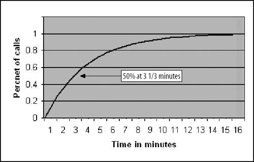

The curve can start at any point in time. At the instant it begins there is no call, so zero percent of the calls happen in zero time. Half the time the next call comes in within 3 1/3 minutes. The next call arrives with 15 minutes nearly all the time. A wait of 16 minutes is possible but almost never occurs.

In this case we are looking at the time interval between events, and this produces an exponential distribution . Excel lets you calculate probabilities in this distribution with the EXPONDIST function.

Before we can use this function we have to calculate a parameter called Lambda . Lambda is the inverse of the average time. So, if our call center gets 3 calls every 10 minutes, the average time between calls is 3.33... minutes. Lambda is 1 divided by 3.33... which equals 0.3. We used minutes to determine Lambda. Therefore, the results we get from the EXPONDIST function will be in minutes.

Suppose we need to know what percentage of the time the next call will arrive within 4 minutes. The formula is:

 =EXPONDIST(4,0.3,TRUE)

The first entry is 4 because we are interested in the 4 minute interval. Next is Lambda (0.3). The option TRUE tells the function that we want the cumulative probability. This returns a value of 0.698. This means that about 70% of the time the next call arrives within 4 minutes.

This distribution looks forward only. It has no memory. This means that even if there has been no call for the last five minutes, there is still a 70% probability that the next call will arrive in the next 4 minutes. The past does not matter, only the future.

1.3.3.3. Gamma distribution

The gamma distribution is similar to the exponential, but more general. It allows you to calculate the probability for multiple events.

We get the same result as with EXPONDIST if we use this formula:

 =GAMMADIST(4,1,3.3333,TRUE)

There are two differences from the EXPONDIST entries. In this case Lambda is 0.3, but the GAMMADIST function requires 1/Lambda. The entry is 3.3333. The 1 is the number of occurrences we want. Here we are interested in the next call, so just one call is involved. If we need to know the probability of getting three calls in the next four minutes, we would enter the formula like this:

 =GAMMADIST(4,3,3.3333,TRUE)

This formula returns a value of 0.1205. There is a 12% chance of getting three calls in the next four minutes.

The GAMMAINV function lets you go the other way. If we want to be 90% sure that the next call will arrive in a certain number of minutes, the formula is:

 =GAMMAINV(0.9,1,3.333)

The 0.9 is the probability we want, and the number of occurrences is one, and 1 divided by Lambda is 3.333. The result is 7.67. That means that there is a 90% chance that the next call will come in during the next 7.67 minutes.

1.3.3.4. Binomial distribution

Some things have only two possible outcomes. A coin toss is heads or tails, a collections call is successful or not, a new account winds up being uncollectible or it doesn't. For this kind of situation, probability is calculated using a binomial distribution .

If the probability that a collections call will result in a payment is 0.1 and a collector makes 75 calls in a day, what is the probability that the calls will result in exactly 10 payments?

Excel has a function that answers this question. The formula is:

 =BINOMDIST(10,75,0.1,TRUE)

The ten is the number of calls we are looking for. There are 75 calls made, and the probability of success on each call is 0.1. The option TRUE tells the function that we want the probability.

The formula returns a value of 0.873. There is an 8.73% chance that exactly 10 payments will come from the 75 calls.

1.3.4. Correlation

Sometimes we need to know if two groups of numbers are related. Correlation is a measure of how much similarity there is between two groups of numbers. If both groups go up or down by the same amount at the same time there is a positive correlation . If they change at the same time but in the opposite direction there is a negative correlation .

Correlation is always a number between one and negative one, and the groups of numbers being tested must have the same numbers of members. In Excel you can calculate correlation using the CORREL function. An example is shown in Figure 1-20.

Here we have two groups of numbers. The formula in cell E1 is:

 =CORREL(A2:A12,B2:B12)

As the first chart illustrates, the numbers, while not equal, tend to move together. The formula returns a value of 0.68. This is a fairly strong correlation and confirms what we see in the chart; the numbers are related. In the bottom chart the numbers are moving at the same time but in the opposite direction. This suggests a negative correlation, and the formula in cell E21 indeed returns a value of -0.805.

Figure 1-20. Positive and negative correlation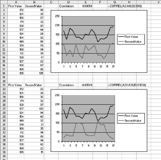

A correlation near zero indicates that the number groups are not related.