6.1 Planning for failure

When designing a reliable data network, network designers are well advised to keep two quotations in mind at all times:

Whatever can go wrong will go wrong at the worst possible time and in the worst possible way . . .

—Murphy

Expect the unexpected.

—Douglas Adams, The Hitchhiker's Guide to the Galaxy

Murphy's Law is widely known and often quoted. While the other directive may appear as humorous nonsense, in practice you should use this to start thinking laterally about failure scenarios you would not normally expect. This exercise can be illuminating.

6.1.1 Terminology

In researching network reliability you will frequently come across terms such as fault tolerance, fault resilience, single/multiple points of failure, and disaster recovery. Differentiating fault tolerance from fault resilience in the literature can be especially difficult, since many vendors use the term "fault tolerance" indiscriminately. In essence, these terms can be defined as follows:

Failure refers to a situation where the observed behavior of a system differs from its specified behavior. A failure occurs because of an error, caused by a fault. The time lapse between the error occurring and the resulting failure is called the error latency [1]. Faults can be hard (permanent) or soft (transient). For example, a cable break is a hard failure, whereas intermittent noise on the line is a soft failure.
Single Point of Failure (SPOF) indicates that a system or network can be rendered inoperable, or significantly impaired in operation, by the failure of one single component. For example, a single hard disk failure could bring down a server; a single router failure could break all connectivity for a network.
Multiple points of failure indicate that a system or network can be rendered inoperable through a chain or combination of failures (as few as two). For example, failure of a single router, plus failure of a backup modem link, could mean that all connectivity is lost for a network. In general it is much more expensive to cope with multiple points of failure and often financially impractical.
Fault tolerance indicates that every component in the chain supporting the system has redundant features or is duplicated. A fault-tolerant system will not fail because any one component fails (i.e., it has no single point of failure). The system should also provide recovery from multiple failures. Components are often overengineered or purposely underutilized to ensure that while performance may be affected during an outage, the system will perform within predictable, acceptable bounds.
Fault resilience implies that at least one of the modules or components within a system is backed up with a spare (e.g., a power supply). This may be in hot standby, cold standby, or load-sharing mode. In contrast with fault-tolerant systems, not all modules or components are necessarily redundant (i.e., there may be several single points of failure). For example, a fault-resilient router may have multiple power supplies but only one routing processor. By definition, one fault-resilient component does not make the entire system fault tolerant.
Disaster recovery is the process of identifying all potential failures, their impact on the system/network as a whole, and planning the means to recover from such failures.

All of these concepts are intimately bound together, and in designing any high-availability solution a rigorous and detailed approach to problem identification and resolution is essential. The designer's goal is to keep the network running no matter what and to maximize the number of failures the network can accommodate without failure while minimizing potential weaknesses. It is also worth restating that high availability does not come cheap. Availability and cost are conflicting constraints on the network design.

6.1.2 Calculating the true cost of downtime

Network designers are largely unfamiliar with financial models [2]. It is, however, imperative in designing reliable networks that the designer gathers some basic financial data in order to cost justify and direct suitable technical solutions. The data may come from line managers or financial support staff and may not be readily collated. Without these data the scale of the problem is undefined, and it will be hard to convince senior financial and operational management that additional features are necessary.

To illustrate the point let us consider a hypothetical consumer-oriented business (such as an airline, car rental, vacation, or hotel reservation call center). The call center is required to be online 24 hours a day, 7 days a week, 365 days a year. The business has 800 staff involved in call handling (transactions), each with an average burdened cost of $25 an hour (i.e., the cost of providing a desk, heating, lighting, phone, data point, etc.). There is a small profit made on each transaction, plus a large profit on any actual sale that can be closed. We assume here that there are on average three sales closed per hour.

Clearly, any downtime represents lost calls, which equates to lost revenue. Worse still, in this kind of operation lost business is typically lost for good, since customers will typically ring a competitor rather than call back later. Our job is to quantify the true cost of downtime and establish what changes to the availability model could improve the situation to the point where the cost of improvements is balanced by acceptable levels of outage. Our starting point would typically be the current network availability. In Figure 6.1 there are four simple cost models, starting with the current availability estimated at 99 percent (i.e., unmanaged). Each of the three subsequent models uses higher availability targets (99.5 percent, 99.9 percent, and 99.99, percent respectively); all other parameters are identical. In Figure 6.1 note that the Cost of Idle Staff is calculated as (Headcount × Burdened Cost × Downtime). Production Losses are calculated as (Headcount × Transactions per Hour X Profit per Transaction X Downtime). Lost Sales are calculated as (Headcount × Sales per Hour × Profit per Sale × Downtime).

Headcount	800	Headcount	800
Burdened Cost/hour	$25	Burdened Cost/hour	$25
Transactions/Hour per Head	40	Transactions/Hour per Head	40
Profit per Transaction	$0.5	Profit per Transaction	$0.5
Sales per Hour per Head	3	Sales per Hour per Head	3
Profit Per Sale	$35	Profit Per Sale	$35

Availability (%)	99.00%	Availability (%)	99.50%
Downtime per Year (hours)	87.60	Downtime per Year (hours)	43.80
Lost Transactions	2,803,200	Lost Transactions	1,401,600

Cost of Idle Staff ($)	$1,752,000	Cost of Idle Staff ($)	$876,000
Production Losses ($)	$1,401,600	Production Losses ($)	$700,800
Lost Sales ($)	$7,358,400	Lost Sales ($)	$3,679,200

TOTAL LOSSES PER YEAR	$10,512,000	TOTAL LOSSES PER YEAR	$5,256,000
(a)		(b)
Headcount	800	Headcount	800
Burdened Cost/hour	$25	Burdened Cost/hour	$25
Transactions/Hour per Head	40	Transactions/Hour per Head	40
Profit per Transaction	$0.5	Profit per Transaction	$0.5
Sales per Hour per Head	3	Sales per Hour per Head	3
Profit Per Sale	$35	Profit Per Sale	$35

Availability (%)	99.90%	Availability (%)	99.99%
Downtime per Year (hours)	8.76	Downtime per Year (hours)	0.88
Lost Transactions	280,320	Lost Transactions	28,032

Cost of Idle Staff ($)	$175,200	Cost of Idle Staff ($)	$17,520
Production Losses ($)	$140,160	Production Losses ($)	$14,016
Lost Sales ($)	$735,840	Lost Sales ($)	$73,584

TOTAL LOSSES PER YEAR	$1,051,200	TOTAL LOSSES PER YEAR	$105,120
(c)		(d)

Figure 6.1: Cost of unavailability in a fictitious call center.

Financial models can be instructive. The current network availability, Figure 6.1(a) predicts nearly four whole days of lost business in any year, equating to $8.5 million projected annual lost business unless additional countermeasures are employed. These hard data can be used as a starting point for justifying a range of network and system enhancements; in many cases even relatively modest enhancements could significantly improve availability. In Figure 6.1(b) we can see that an increase of only 0.5 percent availability reduces predicted losses by 50 percent. Note that the cost of meeting very high availability targets tends to rise dramatically; each business needs to draw the line where it sees fit.

6.1.3 Developing a disaster recovery plan

All networks are vulnerable to disruption. Sometimes these disruptions may come from the most unlikely sources. Natural events such as flooding, fire, lightning strikes, earthquakes, tidal waves, and hurricanes are all possible, as well as fuel shortages, electricity strikes, viruses, hackers, system failures, and software bugs. History shows us that these events do happen regularly. As recently as 1999 and 2000 we saw the seemingly impossible: power shortages in California threatened to cripple Silicon Valley, and a combination of fuel shortages, train safety issues, and massive flooding in the United Kingdom meant that many staff simply could not get to work. In fact, various studies indicate that the majority of system failures can be attributed to a relatively small set of events. These include, in decreasing order of frequency, natural disaster, power failure, systems failure, sabotage/viruses, fire, and human error. There is also a general consensus that companies that take longer than a full business week to get back online run a high risk of being forced out of business entirely (some analysts state as high as 50 percent). For further information on recent disaster studies, see [3, 43].

The first step in mitigating the effects of disaster is to plan for it, especially if you have mission- or business-critical applications running on your network. In order to capture this process you need to create a Disaster Recovery (DR) plan; a general approach to the creation of a DR plan is, as follows:

Benchmark the current design—Perform a full risk assessment for all key systems and the network as a whole. Identify key threats to system and network integrity. Analyze core business requirements and identify core processes and their dependence upon the network. Assign monetary values of loss of service or systems.
Define the requirements—Based on business needs, determine an acceptable recovery window for each system and the network as a whole. If practical specify a worst-case recovery window and a target recovery window. Specify priorities for mission- or business-critical systems.
Define the technical solution—Determine the technical response to these challenges by evaluating alternative recovery models, and select solutions that best meet the business requirements. Ensure that a full cost analysis of each solution is provided, together with the recovery times anticipated under catastrophic failure conditions and lesser degrees of failure.
Develop the recovery strategy—Formulate a crisis management plan identifying the processes to be followed and key personnel response to failure scenarios. Describe where automation and manual intervention are required. Set priorities to clearly identify the order in which systems should be brought back online.
Develop an implementation strategy—Determine how new/additional technology is to be deployed and over what time period. Document changes to the existing design. Identify how new/additional processes and responsibilities are to be communicated.
Develop a test program—Determine how business- and mission-critical systems may be exercised and what the expected results should be. Define procedures for rectifying test failures. Run tests to see if the strategy works; if not, make refinements until satisfied.
Implement continuous monitoring and improvements—Once the disaster recovery plan is established, hold regular reviews to ensure that the plan stays synchronized as the network grows or design features are modified.

Disaster recovery models

There are a number of practical approaches to DR, particularly with respect to protecting valuable user and configuration data. These include tape or CD backup, electronic vaulting, server mirroring, site mirroring, and outsourcing, as follows:

Tape or CD site backup—Tape or CD-ROM backup and restore are the widely used DR methods for sites. Traditionally, key data repositories and configuration files are backed up nightly or every other night. Backup media are transported and securely stored at a different location. This enables complete data recovery should the main site systems be compromised. If the primary site becomes inoperable, the plan is to ship the media back, reboot, and resume normal operations.

Pros and Cons: This is a low-cost solution, but the recovery window could range from a few hours to several days; this may prove unacceptable for many businesses. Media reliability may not be 100 percent and, depending upon the backup frequency, valuable data may be lost.
Electronic vaulting—With remote electronic vaulting, data are archived automatically to tape or CD over the network to a secure remote site. Electronic vaulting ideally requires a dedicated network connection to support large or frequent background data transfers; otherwise, archiving must be performed during off-peak periods or low-utilization periods (e.g., via a nightly backup). Backup procedures can, however, be optimized by archiving only incremental changes since the last archive, reducing both traffic levels and network unavailability.

Pros and Cons: The operating costs for electronic vaulting can be up to four times more expensive than simple tape or CD backup; however, this approach can be entirely automated. Unlike simple media backup there is no requirement to transport backup data physically. Recovery still depends on the most recent backup copy, but this is likely to be more recent due to automation. Electronic vaulting is more reliable and significantly decreases the recovery window (typically, just a few hours).
Data replication/disk mirroring—Remote disk mirroring provides faster recovery and less data loss than remote electronic vaulting. Since data are transferred to disk rather than tape, performance impacts are minimized. With disk mirroring you can maintain a complete replica file system image at the backup site; all changes made to production data are tracked and automatically backed up. Data are typically synchronized in the background, and when the recovery site is initialized or when a failed site comes back online, all data are resynchronized from the replica to production storage. Note that data may be available only in read-only mode at the recovery site if the original site fails (to ensure at least one copy is protected), so services will recover but applications that are required to update data may be somewhat compromised unless some form of local data cache is available until the primary storage comes online. A disk mirroring solution should ideally be able to use a variety of disks using industry-standard interfaces (e.g., SCSI, Fibre Channel, etc.). An example of a disk-mirroring application is IBM's GeoRM [5]. Note that some applications provide data replication services as add-on features of their products (e.g., Oracle, Sybase, DB2, and Domino).

Pros and Cons: Data replication is more expensive than the previous two models, and for large sites considerable traffic volumes can be generated. Ideally, a private storage network should be deployed to separate storage traffic from user traffic. Although more optimal, this requires more maintenance than earlier models.
Server mirroring and clustering—These techniques can be used to significantly reduce the recovery time to acceptable levels. Ideally, servers should be running live and in parallel, distributing load between them but located at different physical locations. If incremental changes are frequently synchronized between servers, then backup could be a matter of seconds, and only a few transactions may be lost (assuming there isn't large-scale telecommunications or power disruption and staff are well briefed on what to do and what not to do in such circumstances). The increasing focus on electronic commerce and large-scale applications such as ERP means that this configuration is becoming increasingly common.

Pros and Cons: This approach is widely used at data centers for major financial and retail institutions but is often too expensive to justify for small businesses. Server mirroring requires more infrastructure to achieve (high-speed wide area links, more routers, more firewalls, and tight management and control systems).
Storage Area Networks (SANs) and Optical Storage Network (OSNs)—There is increasing interest in moving mission- and business-critical data off the main network and offloading it onto a privately managed infrastructure called a Storage Area Network (SAN). Storage can be optically attached via standard high-speed interfaces such as Fibre Channel and SCSI (with optical extenders), providing a physical separation of storage from 600 meters to 10 kilometers. Servers are directly attached to this network (typically via Fibre Channel or ESCON/FICON interfaces [5] and are also attached to the main user network. SANs may be further extended (to thousands of kilometers) via technologies such as Dense Wave Division Multiplexing (DWDM), forming optical storage networks. This allows multiple sites to share storage over reliable high-speed private links.

Pros and Cons: This approach is an excellent model for disaster recovery and storage optimization. It significantly increases complexity and cost (though storage consolidation may recover some of these costs), and it is, therefore, appropriate only for major enterprises at present. One big attraction for many large enterprises is that the whole storage infrastructure can be outsourced to a Storage Service Provider (SSP). This facilitates a very reliable DR model (some providers are currently quoting four-nines (99.99 percent) availability.

As mentioned previously, there are specialized organizations that offer disaster recovery as an outsourced service, including Storage Service Providers (SSPs). Service may include automated response so that key systems on the network are remotely reconfigured or rebooted in the event of failure, through complete service mirroring on their network, so that business can continue even in the event of a total failure of your location. The arguments for and against outsourcing are very much a matter of personal preference and are dependent on the size and type of organization. In-house DR offers more control, potentially lower costs, and tighter security (some organizations may not want data to be seen by a third party). There may be incompatibilities and miscommunication between the staff, systems, and processes used by the outsourcing company and your own; these need to be addressed early on to avoid surprises. Another argument against outsourcing is that under a real disaster situation, the company you have outsourced to will be so busy helping other clients that you may not get the response time you expect (which leads to the ludicrous situation where you might consider having a DR plan to cope with failure of your DR outsourcing company, although cost is likely to prohibit this).

Outsourced DR may be the only sensible option for organizations that either cannot attract skilled IT staff or simply do not want the headache. It is perhaps most appropriate for mainframe scenarios, which are often mission critical, and where skilled operations staff are very hard to come by. To avoid contention, it is perhaps wise to choose one of the major outsourcing companies with an established reputation and the resources to deal with many clients concurrently.

6.1.4 Risk analysis and risk management

Once a basic network design is conceived, one of the major concerns of a network designer is to offer appropriate levels of fault tolerance for key services, systems, and communication links (where "appropriate" is either defined explicitly by the customer or determined against business needs). If you are supplying a network to a customer, from the customer perspective there may be one or more very specific requirements to be met, for example:

There shall be no single point of failure in Equipment Room A.
Service HTTP-2 shall recover from any system failure within 30 seconds.
The routing network shall reconverge around any single point of failure within ten seconds.

A key consideration when planning for high availability, and particularly fault tolerance, is the cost of implementation versus the estimated cost of failure (based on the probability of failure occurring and the duration of downtime prior to recovery). For most organizations, the cost of making a network totally fault tolerant is simply too prohibitive; our real task is to quantify risk and then work out ways of managing it. In terms of network design this is a two-stage process, as follows:

Risk analysis is the process of collecting all relevant facts and assumptions concerning network outages, and then using this information to estimate the probability and financial impact of such outages. This phase should also identify any potential mitigation techniques and quantify their benefits if deployed.
Risk management is the process of taking input from the risk analysis phase and using that information to make decisions about which risks to take (i.e., which mitigation techniques to adopt and which vulnerabilities are deemed to be acceptable risks).

While on paper this seems fairly straightforward, in practice there are a number of issues that make this process more of an art than a science, including the following:

Scope of failure events—Large internetworks are a highly complex mixture of systems and subsystems, and these entities interact with external systems. It is virtually impossible to identify all possible failure scenarios within the bounds of the network, never mind failures caused by external threats such as malicious users. In practice we list only problems that we know about.
Event probability distribution—The distribution pattern of many naturally occurring events can be modeled using statistical techniques such as Gaussian and Poisson models [2]. These rules do not hold true for malicious users, so classical statistical methods are probably inappropriate.
Event independence—As discussed in [2], an important concept used frequently in network modeling is the independence of events. With natural events such as floods or earthquakes we can use classical methods of estimating the probability that two events will occur simultaneously by multiplying their probabilities together. However, malicious user attacks against systems typically involve multiple simultaneous events, often related, and possibly not anticipated. To calculate the joint probabilities of events related in an unknown manner is practically impossible.
Quantifying loss—In practice it is often very difficult to get agreement on the real loss associated with an event after the event has taken place. While there is a substantial body of knowledge on loss valuation available from auditors, different businesses and organizations may place valuations with ranges several orders of magnitude apart.
Scope of mitigation techniques—We cannot exhaustively list all mitigation techniques. There are simply too many permutations, and no single organization has the time or resource to identify all of them.
Quantifying reduction in expected loss—In order to quantify the cost effectiveness of various mitigation techniques, we need to calculate the reduction in expected loss. Unfortunately, there is no universally accepted way to do this with any degree of credibility.
Sensitivity—In practice risk analysis can be very sensitive to detail. For example, a small change in probability or expected loss can influence the choice of one technique over another, and this could have cascading effects on subsequent decisions. Building sensitivity into risk analysis is likely to create a far more complex model.

Much of risk analysis and risk management treat systems as individual entities; however, when things go wrong in networks the failure scenarios are often complex and involve several different systems. We cannot, therefore, assume that system failures are independent, but if we try to calculate all combinations of events and their impacts on all combinations of systems, we are presented with an extremely daunting combinatorial problem. Networking introduces new classes of events and different types of losses and may dramatically change the expected loss reduction associated with different mitigation techniques—and that's just the beginning. This sounds like a classic case for smart software automation; however, there are very few complete packages for analyzing risk in data networks. There are a number of commercial and public domain vulnerability testing tools but very few integrated tools for discovering and quantifying risk. A product called Expert from L-3 Security (now part of Symantec [6]) takes an innovative approach in automatically locating risk and calculating the financial impact; it holds a database of hundreds of known vulnerabilities and thousands of policy safeguards. The downside is that an extensive audit of the network and its systems must be carried out before use; however, this is work that needs to be done never the less.

Regardless of all these seemingly intractable problems and the lack of good tools, it is essential that you perform at least a basic risk assessment. Without this analysis you could overlook critical issues that could be easily remedied. Depending upon the nature of the business, the causes of network or service outages may be easy or hard to quantify. Since we have to start somewhere, the first step is to attempt to identify all critical Single Points of Failure (SPOF).

Identify single points of failure

By analyzing the single points of failure in the network we can make a first stab at quantifying the scope and monetary impact of the most serious failures. This often proves to be a useful and illuminating exercise (the realization that a company's global e-business strategy relies on a flaky four-year-old Ethernet switch can be a moment of purgatory for top executives). Figure 6.2 illustrates a simple network with two sites, the corporate headquarters LAN (Site-A), housing valuable customer database, e-business, and mail services; and a remote depot (Site-B), handling warehousing and dispatch. This network has grown and functions reasonably well but offers little in the way of fault tolerance. Let us assume that the corporate LANs are all switched Ethernet segments, to which a total of 350 users are connected to a single switching concentrator in a central equipment room. At the remote depot, a single Ethernet segment is connected to the corporate headquarters through a single router interface, across a 64-Kbps leased line. Dial-up users can access the router and corporate services via dial-up modem links to an RAS/rotary modem pool at HQ.

click to expand
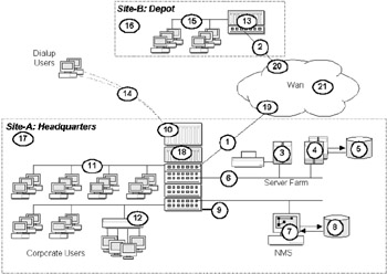
Figure 6.2: Failure analysis of a simple nonresilient design.

Let us determine what the key points of failure are in this design and the effects those failures will have on business operations, as illustrated in Table 6.2. This list is far from exhaustive, but you can begin to see that even with a relatively small network there are many points of failure, some with quite dramatic consequences. Note also that we have only scratched the surface here by identifying the main single points of failure. A more rigorous analysis might identify multiple points of failure in key systems (e.g., failure of two router processes or both power supplies in the HQ router). We may also want to drill down to identify more detailed failure scenarios in the cabling system, failures in connectors or sockets, software failure, disk failures, NVRAM failures, routing failures, and so on.

Table 6.2: Quick Analysis of Major Points of Failure and Their Immediate Effects on the Example Network in Figure 6.2
ID	Failure	Effect
1	HQ Wan link	Loss of all communications to HQ. All e-business activities halted.
2	Remote office Wan link	Loss of all communications to remote Depot
3	Web/Mail server	Loss of printing. Intranet and mail services. All e-business activities halted.
4	Database Server	Partial loss of Intranet services. Impact to Sales, Marketing and Finance
5	Database	Major Impact to Sales. Loss on invoices and status information
6	Server LAN	Loss of all HQ printing, Intranet and mail services. All e-business activities halted.
7	NMS	Loss of all control systems and logging information
8	NMS database	Loss of all configuration, logging and audit information
9	Power to Equipment Room	Total loss of all HQ Services. All e-business activities halted.
10	PAS/Modem Rotary	Loss of all remote dialup access to HQ
11	Corporate LAN	Loss of all user access
12	Terminal Server	Loss of all TN3270 access to parts database at Depot
13	Remote Router	Loss of all communications to remote Depot
14	POTS Failure	Loss of all remote dialup access to HQ
15	Depot LAN	Loss of all depot communications and dispatch operations
16	Depot Site	Loss of all depot operations
17	HQ Site	Loss of all HQ operations and services. All e-business activities halted
18	HQ Firewall-Router	Loss of all external access to HQ. All e-business activities halted.
19	WAN to HQ PoP	Loss of all communications to HQ. All e-business activities halted
20	WAN to Depot PoP	Loss of all communications to Depot. Dispatch activities halted.
21	WAN	Loss of all communications. All e-business activities halted.

The next logical step is to categorize and then estimate the costs of each particular failure. If, for example, we turn over an average $50,000 of new business every hour via the HQ Web server, then failures such as 1 and 18 in Table 6.2 are clearly business critical, and the design will almost certainly require modification to provide server mirroring or hot standby facilities. On the other hand, complete failure of the HQ site (e.g., due to an earthquake or bomb) is more difficult to resolve, since it will require substantial site duplication at a different location, possibly via an outsourced disaster recovery program. Each situation needs to be individually assessed on its relative merits to see if a technological solution is feasible and financially justifiable.

Quantifying risk

Fault-tolerant design is essentially a process of identifying and quantifying risk and then balancing those costs against the cost of protection. Once we understand what the risk is, we can deal with it in one of three ways: accept it, mitigate or reduce it, or transfer it (i.e., accept it but insure against it). Ideally, you need to work through each of the services, resources, and data stores available on the network and logically break down their vulnerability, value, and likelihood of being compromised. You can then start to map out who will be allowed to access these resources and what countermeasures you will put in place to minimize the risk of compromise. You can start by asking the following questions:

How important is the operation of each system/database/link to the business?
What is the monetary value per hour/minute/second in lost revenue if these services/systems are unavailable?
How valuable are the data held on any such devices (i.e., the true cost of replacement)?
What kind of a threat is each resource vulnerable to (disk failure, power failure, denial of service, virus, etc.).
What is the likelihood of these threats occurring (0–100 percent)?
How many times per year would you anticipate such a failure?
What is the likely recovery time for recovering from such failures?

ALE method

It can be instructive to perform a weighted risk analysis by estimating the risk of losing a resource and the value of that resource and then multiplying them together to get a weighted value. This is more formally known as the Annual Loss Expectancy (ALE) method. ALE is a method of quantifying risk by estimating a loss value per incident and then estimating the number of incidents per year to arrive at an Annual Loss Expectancy (ALE). Here, each item at risk produces a Single Loss Expectancy (SLE), calculated as:

SLE = V_x×E_x

where

V_x = the asset value for a specific item, x, expressed as a monetary value (e.g., $35,000, £100,000, DM 200,000)
E_x = exposure factor for a specific item, x, expressed as a percentage (0–100%) of the asset value.

If we are at risk of losing a database through a virus on an unprotected public file server (Table 6.3, item 5), for which we have no backups (worst-case scenario), then the cost to replace it might be calculated as the time to recreate it—say, two man-years at $45,000. Given the scenario painted, we could probably assume that the database risk is 75 percent, giving us an SLE of (2 × 45 × 75%)—that is, $67.5K. Note that the manpower cost would almost certainly be higher, since we have not accounted for the true burdened costs (heating, space, expenses, etc.) plus possible lost productivity for other projects for the duration of this fix.

Table 6.3: ALE Analysis of Major Points of Failure
ID	Failure	Asset Value	Exposure Factor	SLE	Annual Occurance	ALE
1	HQ Wan link	$250,000	80%	$200,000	2.5	$500,000
2	Remote office Wan link	$15,000	75%	$11,250	3.0	$33,750
3	Web/Mail server	$250,000	75%	$187,500	4.0	$750,000
4	Databa e Server	$100,000	20%	$20, 000	3.0	$60,000
5	Database	$90,000	75%	$67,500	2.0	$135,000
6	Server LAN	$20,000	25%	$5,000	4 0	$20,000
7	NMS	$10,000	10%	$1,000	3.0	$3,000
8	NMS database	$5,000	10%	$500	2.0	$1,000
9	Power to Equipment Room	$9,000	15%	$1,350	2.0	$2,700
10	PAS/Modem Rotary	$10,000	90%	$9,000	3.0	$27,000
11	Corporate LAN	$25,000	50%	$12,500	4.0	$50,000
12	Terminal Server	$5,000	20%	$1,000	0.5	$500
13	Remote Router	$200,000	75%	$150,000	1.5	$225,000
14	POTS Failure	$20,000	50%	$10,000	3.0	$30,000
15	Depot LAN	$200,000	75%	$150,000	2.0	$300,000
16	Depot Site	$100,000	90%	$90,000	1.0	$90,000
17	HQ Site	$250,000	90%	$225,000	1.0	$225,000
18	HQ Firewall-Router	$40,000	50%	$20,000	0.3	$5,000
19	WAN to HQ PoP	$100,000	10%	$10,000	1.0	$10,000
20	WAN to Depot PoP	$25,000	10%	$2,500	1.0	$2,500
21	WAN	$50,000	75%	$37,500	0.5	$18,750

To get an annualized SLE (i.e., an ALE) we simply factor in the predicted number of times that such an event will occur over a year, using the formula:

ALE = SLE × N_x,

where

N_x = the annual rate of occurrence for a specific event, x.

Using the previous SLE illustration, if we expect to have a virus attack on our database twice in a year then the ALE for database loss is $135,000. Table 6.3 illustrates how all of the failures listed in Table 6.2 might be quantified using the ALE method. The ALE column can be used as a guide to rank the areas of the design requiring most attention.

Determine recovery times

Once we have identified all single points of failure and quantified risk, we need to determine the likely failure times and the baseline time to fix or recovery time. Whether the fix is automatic or requires manual intervention, you should have answers to the following questions for each failure identified:

How are maintenance staff notified about a problem? Do monitoring tools alert you to the problem proactively, or are panic calls from users the first sign of trouble?
How long will it take to track down the cause of the problem for each failed system or component?
Does the design of the network naturally assist you in focusing on the problem quickly?
What happens if a failure occurs outside of business hours? How does that affect recovery times?
How are problems typically resolved for each system (remote reboot, reconfiguration, engineer on site)?
Are spares held, if so where, and who controls them?
Are backup configurations maintained? If so, how are they deployed in an emergency?

Without good management diagnostic tools and well-defined procedures, tracking down and resolving problems could conceivably take many hours, and most organizations simply cannot tolerate this level of downtime. Many companies are now relying on their networks as mission-critical business tools, and network downtime could seriously impact both profitability and credibility in the marketplace. As networks become even more tightly integrated and networking software enables files to be more readily distributed, the proliferation of computer viruses is becoming a major issue for maintaining network availability. Viruses such as the ILOVEYOU worm caused widespread chaos at many sites during 2000.

Managing risk

Risk management is the process of making decisions about which risks to take, which risks to avoid, and which risks to mitigate. Risk management is, therefore, a compromise; ultimately money must be spent to mitigate risk, and money may be lost if risks are accepted. Since the output of the risk analysis process can never be flawless, risk management relies on a mixture of common sense and business and basic accounting skills. One of the problems during the risk management phase is that the people making these decisions often may understand very little of the technology. It is, therefore, important that the risk analysis process should reduce the expression of each risk element to its most fundamental and understandable form, so that it can be translated directly into business terms. For example:

If the HTTP Server (WSELL_2A) loses software integrity, then all pending transactions may be lost and new sessions cannot be serviced because the Telnet daemon may have locked.

should be translated as:

If the main Web server dies, then no new customers will be able to buy products until it is rebooted, and we are likely to lose data from some of the sales calls in process at the point of failure.

A pragmatic and widely used technique in risk management is the covering technique. This involves listing all anticipated attacks and all possible defenses and then attempting to match appropriate defenses with each attack. Each defensive technique is assessed using a qualitative statement about its effectiveness. The risk manager then decides which attacks to protect against and which not to, based on a subjective view on the impact of each attack on the organization. Clearly, given the absence of numerical data, the risk manager has a great deal of latitude and must consider facts from many different sources in order to reach good decisions (it also implies that you need to choose a good risk manager!).

The following are some approaches we might consider to mitigate the types of failures we have identified in our example network:

Install a second firewall router at the HQ site, mesh link both routers into the two switches, and then mesh link to both firewalls. Run a fast routing protocol such as OSPF or EIGRP on the internal interfaces of the corporate routers to ensure rapid convergence around failures. Make use of any load-balancing features available, if appropriate.
Install a backup ISDN link from the remote site to the second HQ router. Configure the ISDN device to auto-dial whenever loss of WAN service is detected at either site.
Add a second server farm with duplicate servers on a different segment, meshed into the two switches and then into the two firewalls. Front end these servers with a load-balancing device, or use a load-sharing dynamic protocol between the servers, such as HSRP or VRRP.
Install disk mirroring in key servers and the firewall to protect against hard disk failure.
Install a UPS at HQ to cover at least four hours of downtime. Consider DC backup via a diesel generator if justified.

The cost of each solution should reflect both the product cost and the cost of deployment. Most of these solutions are straightforward to analyze; however, they become increasingly difficult to cost justify as we work down the list. You need to balance the risk of component or system failure (using data such as MTBF/MTTR) against the scope and monetary impact of downtime due to that particular failure. A failure that affects a single user is unlikely to rate highly, even if the effect is complete downtime for that user.

Whichever model you use, these types of data can be used in financial planning projects when attempting to justify expenditure on fault-tolerant features, and it certainly helps to focus attention on critical vulnerabilities. If the annual projected losses due to system or network component failures exceed the cost of the preventative measures, then it should be easier to convince senior managers to allocate budgets accordingly. Just be aware that much of this process boils down to good judgment, regardless of the number of decimal points your analysis produces.

6.1.5 Availability analysis

In any network it is useful to have some way of quantifying availability and reliability, since this will determine how much money should be spent on avoiding loss of service and where that money should be targeted.

Quantifying availability

A simple way of expressing availability is to use the percentage uptime that a system or service offers, calculated as:

A% = Operational Time/Total Time

where time is normally expressed in hours. For example, consider a router that fails only once during the year and requires three hours to fix. Availability is calculated as:

A% = [(365 × 24) - 3)]/(365 x 24)
A% = 99.966%

Typical availability values range between 95 percent and 99.99999 percent, depending upon whether a best-effort or carrier-class service is required (as a result, carrier class is often referred to as seven-nines availability). While 95 percent uptime may sound pretty good, it is generally unacceptable for most working networks, since it translates to an average 1.2 hours of network outages per day (as illustrated in Table 6.4). To calculate the availability in hours, use the formula [8,760 × (1 - Availability%)], where 8,760 is the number of hours in a 365-day year. System classification taken from [7].

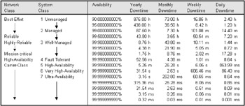
Table 6.4: Availability Expressed as a Percentage Off Uptime (Hours = H, Minutes = M, Seconds = S, Milliseconds = MS)

Wide area digital circuits are typically quoted at least 99.5 percent availability, while analog circuits are quoted at 99.4 percent availability. Highly reliable systems should be available at least 99.9 percent of the time, and most reliable networks operate at approximately 99.95 percent availability, with just over five minutes of downtime per week on average. Public operator networks (so-called carrier class networks) may offer availability from 99.99 percent through to 99.999 percent, although in practice this level of availability may be very expensive to deploy and will usually rely on highly redundant design with a mixture of hot-standby components and clustered solutions. Cost and complexity are the main barriers in moving beyond this level of availability, and increased complexity is itself a contributing factor in reducing reliability.

Availability can be expressed mathematically, using a number of components as input, as follows:

Mean Time Between Service Outages (MTBSO) or Mean Time Between Failure (MTBF) is the average time (expressed in hours) that a system has been working between service outages and is typically greater than 2,000 hours. Since modern network devices may have a short working life (typically five years), MTBF is often a predicted value, based on stress-testing systems and then forecasting availability in the future. Devices with moving mechanical parts such as disk drives often exhibit lower MTBFs than systems that use fixed components (e.g., flash memory). Example MTBFs for a range of network devices are shown in Table 6.5.

Table 6.5: Example MTBFs for Real Network Devices
Component	MTBF hours	MTBF years
Managed Repeater Chassis/Backplane	895,175	102.2
Fibre Optic IO Module (chassis based)	236,055	26.9
UTP IO Module (chassis based)	104,846	12.0
Management Module (chassis based)	75,348	8.6
Power Supply	44,000	5.0
Ethernet Transceiver	250,000	28.5
Terminal Server (standalone)	92,250	10.5
Remote Bridge (standalone)	41,000	4.7
Firewall (1 hard drive, 4 * IO card, no CDROM, no Floppy)	36,902	4.2
ATM Switch (3 * IO cards)	54,686	6.2
ATM Switch (16 * IO cards)	34,197	3.9
X.25 Triple-X PAD (standalone)	41,000	4.7
X.25 packet Switch (standalone)	6,000	0.7
Statistical Multiplexer (standalone)	5,300	0.6

Mean Time To Repair (MTTR) is the average time to repair systems that have failed and is usually several orders of magnitude less that MTBF. MTTR values may vary markedly, depending upon the type of system under repair and the nature of the failure. Typical values range from 30 minutes through to 3 or 4 hours. A typical MTTR for a complex system with little inherent redundancy might be several hours.

In effect, MTBF and MTBSO both represent uptime, whereas MTTR represents downtime. As a general rule, an MTTR of less than one hour and an MTBF of more than 4,000 hours is considered good reliability, since it translates to two failures a year, with a total average yearly downtime of two hours (i.e., better than 99.98 percent availability). Note, however, that all of these factors represent average values (you could be unlucky and have two or more failures in the first month!). Note also that vendors may quote MTTR values assuming an engineer is already on site; you must also take into account any significant delays in the engineer getting to site from the time the fault call is logged. This may significantly increase the final MTTR and could result in different MTTRs for the same piece of equipment at different sites, depending upon their location and reachability. To simplify matters you may want to take the average MTTR for all of your sites.

Quantifying availability for discrete systems

Simply put, availability is the length of time a system is working compared with the expected lifetime of that system. Availability, A, and its complement, unavailability, U, are calculated as follows (where n is the system number):

A_n = MTBF_n/(MTBF_n + MTTR_n) × 100
U_n= 1- [MTBF_n/(MTBF_n + MTTR_n)] × 100

The first equation is effectively the same as dividing operational time by total time, as presented previously. Another way of looking at unavailability is that it represents the probability of failure. The average number of failures, F, in a given time, T hours, is calculated as:

F_n = T/(MTBF_n + MTTR_n)

These methods of quantifying availability are more granular than a simple percentage in that they estimate both the frequency and the duration of system or network outages. For example, a low MTBF of 2,500 hours and an MTTR of 30 minutes indicate that there will be on average 3.5 failures in a year (T = 8,760 hours), or one failure every 3.4 months. In each case the downtime is expected to last about 30 minutes (i.e., the MTTR). A better MTBF, say 46,000 hours, indicates only 0.1904 failures per year, or one failure every 5.25 years.

Reliability

Reliability can be defined as the distribution of time between failures, and is often specified by the MTBF for Markovian failures [2]. Reliability, R, is specified as the probability that a system will not fail before T hours have elapsed:

R = e^-^t^/MTBF

For example, assume a system with an MTBF of 32,000 hours and a time, T, of one year (8,760 hours); this gives a reliability of 76.05 percent. If we increase the MTBF (say by selecting an alternate system) to 52,000 hours, this increases the reliability to 84.50 percent. For a network of systems in series we can calculate the total reliability, R_t, as follows:

Rt = e^-t^{[(1/MTBF1+(1/MTBF2)+(1/MTBF3)]}

For example, if we had three systems in series with MTBFs of 26,000, 42,000, and 56,000 hours, respectively, the overall reliability for a year would be 49.56 percent.

Quantifying availability in networked systems

Networked systems in series

For a network of devices in series, the total availability, A_t, is calculated as the product of all availabilities:

Consider the example network in Figure 6.3. We have two switches and two routers in series; both sites are in very remote locations.

click to expand
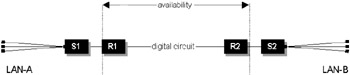
Figure 6.3: Point-to-point network in series.

Let us assume that the router MTBF is 8,725 hours. The MTTR is calculated as 35 hours (1 hour call logging, 30 hours to ship parts and fly in an engineer, 4 hours to fix); hence, the router availability is 8,725/(8725 + 35) × 100, giving 99.6 percent. The service provider quotes the circuit availability at 99.5 percent. For the purpose of this example we are only interested in the router point-to-point link, so we can calculate the total availability as:

A_t = (0.996 × 0.996 × 0.995) × 100
A_t = 98.71%

Notice that the final result is lower than any of the individual components, as one would expect.

Networked systems in parallel

If we now modify the design to add a second parallel link in parallel, as illustrated in Figure 6.4, we can calculate the total availability as:

click to expand
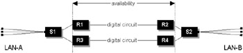
Figure 6.4: Point-to-point network in parallel.

where

j = the number of paths

i = the number of devices in series along those paths.

We can simplify this calculation by first working out the total availability for each path using the equation for solving availability in series. In this case we know from the previous work that this is 98.71 percent for each path. Substituting this result for this example we arrive at the following:

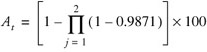
A_t = (1-0.0129²) × 100
A_t = 99.98%

Notice that the final result is higher than any of the individual components, as one would expect. Availability improves with parallel networks as we add more parallel systems; the converse is true of systems in series.

Combining systems in parallel and in series

To calculate availability for hybrid system, simply work out all the parallel systems first and then treat the whole system as if it were a network in series. For example, in the network illustrated in Figure 6.4, we might want to calculate the end-to-end availability, including the switch and intermediate LAN links. Let us assume that the switches offer 99.7 percent availability, and the LAN cross-connects to the routers offer 99.6 percent availability. We have already calculated the availability of the two parallel paths, so the final calculation is simply a network in series:

A_t = (0.996 × 0.997 × 0.9998 × 0. 997 × 0.996) × 100
A_t = 98.59%

In summary, with any network design and particularly those with mission- or business-critical data and services, the design must be examined from the top down, starting with the wide area circuit design right down to the component level, identifying all probable single points of failures. There should be a well-defined and documented action plan for analyzing and resolving potential failures, either automatically or manually. Ultimately, networks should be able to heal themselves without requiring human intervention, but today this is not really achievable cost effectively.

The following sections illustrate the technologies and techniques available today to design fault-tolerant networks. These techniques are contrasted and their relative strengths and weaknesses assessed. For further information on risk analysis, the interested reader is directed to [8, 9].